Postprocessing computations
As the final theme in this chapter, we will look at how to postprocess computations; that is, how to compute various derived quantities from the computed solution of a PDE. The solution \( u \) itself may be of interest for visualizing general features of the solution, but sometimes one is interested in computing the solution of a PDE to compute a specific quantity that derives from the solution, such as, e.g., the flux, a point-value, or some average of the solution.
Test problem
As a test problem, we consider again the variable-coefficient Poisson problem with a single Dirichlet boundary condition: $$ \begin{alignat}{2} - \nabla\cdot(\kappa\nabla u) &= f \quad &&\mbox{in } \Omega, \tag{5.1} \\ u &= \ub \quad &&\mbox{on}\ \partial\Omega\tp \end{alignat} $$ Let us continue to use our favorite solution \( u(x,y)=1+x^2+2y^2 \) and then prescribe \( \kappa(x,y)=x+y \). It follows that \( \ub(x,y) = 1 + x^2 + 2y^2 \) and \( f(x,y)=-8x-10y \).
As before, the variational formulation for this model problem can be specified in FEniCS as
a = kappa*dot(grad(u), grad(v))*dx
L = f*v*dx
with the coefficient \( \kappa \) and right-hand side \( f \) given by
kappa = Expression('x[0] + x[1]', degree=1)
f = Expression('-8*x[0] - 10*x[1]', degree=1)
Flux computations
It is often of interest to compute the flux \( Q = -\kappa\nabla u \). Since \( u = \sum_{j=1}^N U_j \phi_j \), it follows that $$ \begin{equation*} Q = -\kappa\sum_{j=1}^N U_j \nabla \phi_j\tp \end{equation*} $$ We note that the gradient of a piecewise continuous finite element scalar field is a discontinuous vector field since the basis functions \( \{\phi_j\} \) have discontinuous derivatives at the boundaries of the cells. For example, using Lagrange elements of degree 1, \( u \) is linear over each cell, and the gradient becomes a piecewise constant vector field. On the contrary, the exact gradient is continuous. For visualization and data analysis purposes, we often want the computed gradient to be a continuous vector field. Typically, we want each component of \( \nabla u \) to be represented in the same way as \( u \) itself. To this end, we can project the components of \( \nabla u \) onto the same function space as we used for \( u \). This means that we solve \( w = \nabla u \) approximately by a finite element method, using the same elements for the components of \( w \) as we used for \( u \). This process is known as projection.
Projection is a common operation in finite element analysis and, as
we have already seen, FEniCS
has a function for easily performing the projection:
project(expression, W), which returns the projection of some
expression into the space W.
In our case, the flux \( Q = -\kappa\nabla u \)
is vector-valued and we need to pick W as the vector-valued function
space of the same degree as the space V where u resides:
V = u.function_space()
mesh = V.mesh()
degree = V.ufl_element().degree()
W = VectorFunctionSpace(mesh, 'P', degree)

grad_u = project(grad(u), W)
flux_u = project(-k*grad(u), W)
The applications of projection are many, including turning discontinuous gradient fields into continuous ones, comparing higher- and lower-order function approximations, and transforming a higher-order finite element solution down to a piecewise linear field, which is required by many visualization packages.
Plotting the flux vector field is naturally as easy as plotting anything else:
plot(flux_u, title='flux field')

flux_x, flux_y = flux_u.split(deepcopy=True)  # extract components
plot(flux_x, title='x-component of flux (-kappa*grad(u))')
plot(flux_y, title='y-component of flux (-kappa*grad(u))')
The deepcopy=True argument signifies a deep copy, which is
a general term in computer science implying that a copy of the data is
returned. (The opposite, deepcopy=False,
means a shallow copy, where
the returned objects are just pointers to the original data.)
For data analysis of the nodal values of the flux field, we can
grab the underlying numpy arrays (which demands a deepcopy=True
in the split of flux):
flux_x_nodal_values = flux_x.vector().dofs()
flux_y_nodal_values = flux_y.vector().dofs()
The degrees of freedom of the flux_u vector field can also be
reached by
flux_u_nodal_values = flux_u.vector().array()
However, this is a flat numpy array containing the degrees of
freedom for both the \( x \) and \( y \) components of the flux and the
ordering of the components may be mixed up by FEniCS in order to
improve computational efficiency.
The function demo_flux in the program
ft10_poisson_extended.py
demonstrates the computations described above.
project to project a finite element
function, it can be instructive to look at how to formulate the
projection mathematically and implement its steps manually in FEniCS.
Let's say we have an expression \( g = g(u) \) that we want to project into some space \( W \). The mathematical formulation of the (\( L^2 \)) projection \( w = P_W g \) into \( W \) is the variational problem $$ \begin{equation} \int_{\Omega} w v \dx = \int_{\Omega} g v \dx \tag{5.2} \end{equation} $$ for all test functions \( v\in W \). In other words, we have a standard variational problem \( a(w, v) = L(v) \) where now $$ \begin{align} a(w, v) &= \int_\Omega w v \dx, \tag{5.3}\\ L(v) &= \int_\Omega g v \dx\tp \tag{5.4} \end{align} $$ Note that when the functions in \( W \) are vector-valued, as is the case when we project the gradient \( g(u) = \nabla u \), we must replace the products above by \( w\cdot v \) and \( g\cdot v \).
The variational problem is easy to define in FEniCS.
w = TrialFunction(W)
v = TestFunction(W)

a = w*v*dx  # or dot(w, v)*dx when w is vector-valued
L = g*v*dx  # or dot(g, v)*dx when g is vector-valued
w = Function(W)
solve(a == L, w)
The boundary condition argument to solve is dropped since there are
no essential boundary conditions in this problem.
Computing functionals
After the solution \( u \) of a PDE is computed, we occasionally want to compute functionals of \( u \), for example, $$ \begin{equation} {1\over2}||\nabla u||^2 = {1\over2}\int_\Omega \nabla u\cdot \nabla u \dx, \tag{5.5} \end{equation} $$ which often reflects some energy quantity. Another frequently occurring functional is the error $$ \begin{equation} ||\uex-u|| = \left(\int_\Omega (\uex-u)^2 \dx\right)^{1/2}, \tag{5.6} \end{equation} $$ where \( \uex \) is the exact solution. The error is of particular interest when studying convergence properties of finite element methods. Other times, we may instead be interested in computing the flux out through a part \( \Gamma \) of the boundary \( \partial\Omega \), $$ \begin{equation} F = -\int_\Gamma \kappa\nabla u\cdot n \ds, \tag{5.7} \end{equation} $$ where \( n \) is the outward-pointing unit normal on \( \Gamma \).
All these functionals are easy to compute with FEniCS, as we shall see in the examples below.
Energy functional
The integrand of the energy functional (5.5) is described in the UFL language in the same manner as we describe weak forms:
energy = 0.5*dot(grad(u), grad(u))*dx
E = assemble(energy)
The functional energy is evaluated by calling the assemble
function that we have previously used to assemble matrices and
vectors. FEniCS will recognize that the form has ''rank 0'' (since it
contains no trial and test functions) and return the result as a
scalar value.
Error functional
The functional (5.6) can be computed as follows:
error = (u_e - u)**2*dx
E = sqrt(abs(assemble(error)))
The exact solution \( \uex \) is here represented by a Function or
Expression object u_e, while u is the finite element
approximation (and thus a Function). Sometimes, for very small
error values, the result of assemble(error) can be a (very small)
negative number, so we have used abs in the expression for E above
to ensure a positive value for the sqrt function.
As will be explained and demonstrated in the section Computing convergence rates, the integration of (u_e - u)**2*dx
can result in too optimistic convergence rates unless one is careful
how the difference u_e - u is evaluated. The general recommendation
for reliable error computation is to use the errornorm function:
E = errornorm(u_e, u)
Flux Functional
To compute flux integrals like \( F = -\int_\Gamma \kappa\nabla u\cdot n \ds \), we need to define the \( n \) vector, referred to as a facet normal in FEniCS. If the surface domain \( \Gamma \) in the flux integral is the complete boundary, we can perform the flux computation by
n = FacetNormal(mesh)
flux = -k*dot(grad(u), n)*ds
total_flux = assemble(flux)
Although grad(u) and nabla_grad(u) are interchangeable in the above
expression when u is a scalar function, we have chosen to write
grad(u) because this is the right expression if we generalize the
underlying equation to a vector PDE. With nabla_grad(u) we
must in that case write dot(n, nabla_grad(u)).
It is possible to restrict the integration to a part of the boundary
by using a mesh function to mark the relevant part, as explained in
the section Setting multiple Dirichlet, Neumann, and Robin conditions. Assuming that the part corresponds
to subdomain number i, the relevant syntax for the variational
formulation of the flux is -k*dot(grad(u), n)*ds(i).
Expressions must be defined using
a particular degree. The degree tells FEniCS into which local
finite element space the expression should be interpolated when
performing local computations (integration). As an illustration,
consider the computation of the integral \( \int_0^1 \cos x \dx = \sin
1 \). This may be computed in FEniCS by
mesh = UnitIntervalMesh(1)
I = assemble(Expression('cos(x[0])', degree=degree)*dx(domain=mesh))
Note that we must here specify the argument domain=mesh to the
measure dx. This is normally not necessary when defining forms
in FEniCS but is necessary here since cos(x[0]) is not associated
with any domain (as is the case when we integrate a Function
from some FunctionSpace defined on some Mesh).
Varying the degree between 0 and 5, the value of \( |\sin(1) - I| \) is
0.036,
0.071,
0.00030,
0.00013,
4.5E-07, and
2.5E-07.
FEniCS also allows expressions to be expressed directly as part of
a form. This requires the creation of a SpatialCoordinate.
In this case, the accuracy is dictated by the accuracy of the
integration, which may be controlled by a degree argument to
the integration measure dx. The degree argument specifies
that the integration should be exact for polynomials of that degree.
The following code snippet shows how to compute the integral \( \int_0^1 \cos x \dx \) using this approach:
mesh = UnitIntervalMesh(1)
x = SpatialCoordinate(mesh)
I = assemble(cos(x[0])*dx(degree=degree))
Varying the degree between 0 and 5, the value of \( |\sin(1) - I| \) is
0.036,
0.036,
0.00020,
0.00020,
4.3E-07,
4.3E-07.
Note that the quadrature degrees are only available for
odd degrees so that degree \( 0 \) will use the same quadrature
rule as degree \( 1 \),
degree \( 2 \) will give the same quadrature rule as degree \( 3 \) and so on.
Computing convergence rates
A central question for any numerical method is its convergence rate: how fast does the error approach zero when the resolution is increased? For finite element methods, this typically corresponds to proving, theoretically or empirically, that the error \( e = \uex - u \) is bounded by the mesh size \( h \) to some power \( r \); that is, \( \|e\| \leq C h^r \) for some constant \( C \). The number \( r \) is called the convergence rate of the method. Note that different norms, like the \( L^2 \)-norm \( \|e\| \) or \( H^1_0 \)-norm \( \|\nabla e\| \) typically have different convergence rates.
To illustrate how to compute errors and convergence rates in FEniCS,
we have included the function compute_convergence_rates in the
tutorial program
ft10_poisson_extended.py.
This is a tool that is very handy when verifying finite element codes
and will therefore be explained in detail here.
Computing error norms
As we have already seen, the \( L^2 \)-norm of the error \( \uex - u \) can be implemented in FEniCS by
error = (u_e - u)**2*dx
E = sqrt(abs(assemble(error)))
As above, we have used abs in the expression for E above to ensure
a positive value for the sqrt function.
It is important to understand how FEniCS computes the error from the
above code, since we may otherwise run into subtle issues when using
the value for computing convergence rates. The first subtle issue is
that if u_e is not already a finite element function (an object created
using Function(V)), which is the case if u_e is defined as an
Expression, FEniCS must interpolate u_e into some local finite
element space on each element of the mesh. The degree used for the
interpolation is determined by the mandatory keyword argument to the
Expression class, for example:
u_e = Expression('sin(x[0])', degree=1)
This means that the error computed will not be equal to the actual error \( \|\uex - u\| \) but rather the difference between the finite element solution \( u \) and the piecewise linear interpolant of \( \uex \). This may yield a too optimistic (too small) value for the error. A better value may be achieved by interpolating the exact solution into a higher-order function space, which can be done by simply increasing the degree:
u_e = Expression('sin(x[0])', degree=3)
The second subtle issue is that when FEniCS evaluates the expression
(u_e - u)**2, this will be expanded into u_e**2 + u**2 -
2*u_e*u. If the error is small (and the solution itself is of
moderate size), this calculation will correspond to the subtraction of
two positive numbers (u_e**2 + u**2 \( \sim 1 \) and 2*u_e*u \( \sim
1 \)) yielding a small number. Such a computation is very prone to
round-off errors, which may again lead to an unreliable value for the
error. To make this situation worse, FEniCS may expand this
computation into a large number of terms, in particular for higher
order elements, making the computation very unstable.
To help with these issues, FEniCS provides the built-in function
errornorm which computes the error norm in a more intelligent
way. First, both u_e and u are interpolated into a higher-order
function space. Then, the degrees of freedom of u_e and u are
subtracted to produce a new function in the higher-order function
space. Finally, FEniCS integrates the square of the difference
function and then takes the square root to get the value of the error
norm. Using the errornorm function is simple:
E = errornorm(u_e, u, normtype='L2')
It is illustrative to look at a short implementation of errornorm:
def errornorm(u_e, u):
    V = u.function_space()
    mesh = V.mesh()
    degree = V.ufl_element().degree()
    W = FunctionSpace(mesh, 'P', degree + 3)
    u_e_W = interpolate(u_e, W)
    u_W = interpolate(u, W)
    e_W = Function(W)
    e_W.vector()[:] = u_e_W.vector().array() - u_W.vector().array()
    error = e_W**2*dx
    return sqrt(abs(assemble(error)))
Sometimes it is of interest to compute the error of the
gradient field: \( ||\nabla (\uex-u)|| \),
often referred to as the \( H^1_0 \) or \( H^1 \) seminorm of the error.
This can either be expressed as above, replacing the expression for
error by error = dot(grad(e_W), grad(e_W))*dx, or by calling
errornorm in FEniCS:
E = errornorm(u_e, u, norm_type='H10')
Type help(errornorm) in Python for more information about available
norm types.
The function compute_errors in
ft10_poisson_extended.py
illustrates the computation of various error norms in FEniCS.
Computing convergence rates
Let's examine how to compute convergence rates in FEniCS.
The solver function in
ft10_poisson_extended.py
allows us to easily compute solutions for finer and finer meshes and
enables us to study the convergence rate. Define the element size
\( h=1/n \), where \( n \) is the number of cell divisions in the \( x \) and \( y \)
directions (n = Nx = Ny in the code). We perform experiments with
\( h_0>h_1>h_2>\cdots \) and compute the corresponding errors \( E_0, E_1,
E_2 \) and so forth. Assuming \( E_i=Ch_i^r \) for unknown constants \( C \) and
\( r \), we can compare two consecutive experiments, \( E_{i-1}=Ch_{i-1}^r \)
and \( E_i=Ch_i^r \), and solve for \( r \):
$$
\begin{equation*}
r = {\ln(E_i/E_{i-1})\over\ln (h_i/h_{i-1})}\tp
\end{equation*}
$$
The \( r \) values should approach the expected convergence rate
(typically the polynomial degree + 1 for the \( L^2 \)-error) as \( i \)
increases.
The procedure above can easily be turned into Python code. Here
we run through a list of element degrees (\( \mathsf{P}_1 \),
\( \mathsf{P}_2 \), and \( \mathsf{P}_3 \)),
perform experiments over a series of refined meshes, and for
each experiment report the six error types as returned by compute_errors.
Test problem
To demonstrate the computation of convergence rates, we pick an exact solution \( \uex \), this time a little more interesting than for the test problem in the chapter Fundamentals: Solving the Poisson equation: $$ \begin{equation*} \uex(x,y) = \sin(\omega\pi x)\sin(\omega\pi y). \end{equation*} $$ This choice implies \( f(x,y)=2\omega^2\pi^2 u(x,y) \). With \( \omega \) restricted to an integer, it follows that the boundary value is given by \( \ub=0 \).
We need to define the appropriate boundary conditions, the exact solution, and the \( f \) function in the code:
def boundary(x, on_boundary):
    return on_boundary

bc = DirichletBC(V, Constant(0), boundary)

omega = 1.0
u_e = Expression('sin(omega*pi*x[0])*sin(omega*pi*x[1])',
                 degree=6, omega=omega)

f = 2*pi**2*omega**2*u_e
Experiments
An implementation of the computation of the convergence rate can be
found in the function demo_convergence_rates in the demo program
ft10_poisson_extended.py.
We achieve some interesting results.
Using the infinity norm of the difference of the degrees of freedom,
we obtain the following table:
| element | \( n=8\ \) | \( n=16\ \) | \( n=32\ \) | \( n=64\ \) |
| \( \mathsf{P}_1 \) | 1.99 | 2.00 | 2.00 | 2.00 |
| \( \mathsf{P}_2 \) | 3.99 | 4.00 | 4.00 | 4.01 |
| \( \mathsf{P}_3 \) | 3.95 | 3.99 | 3.99 | 3.92 |
An entry like 3.99 for \( n=32 \) and \( \mathsf{P}_3 \) means that we estimate the rate 3.99 by comparing two meshes, with resolutions \( n=32 \) and \( n=16 \), using \( \mathsf{P}_3 \) elements. Note the superconvergence for \( \mathsf{P}_2 \) at the nodes. The best estimates of the rates appear in the right-most column, since these rates are based on the finest resolutions and are hence deepest into the asymptotic regime (until we reach a level where round-off errors and inexact solution of the linear system starts to play a role).
The \( L^2 \)-norm errors computed using the FEniCS
errornorm function show the
expected \( h^{d+1} \) rate for \( u \):
| element | \( n=8\ \) | \( n=16\ \) | \( n=32\ \) | \( n=64\ \) |
| \( \mathsf{P}_1 \) | 1.97 | 1.99 | 2.00 | 2.00 |
| \( \mathsf{P}_2 \) | 3.00 | 3.00 | 3.00 | 3.00 |
| \( \mathsf{P}_3 \) | 4.04 | 4.02 | 4.01 | 4.00 |
However, using (u_e - u)**2 for the error computation, with the same
degree for the interpolation of u_e as for u, gives strange
results:
| element | \( n=8\ \) | \( n=16\ \) | \( n=32\ \) | \( n=64\ \) |
| \( \mathsf{P}_1 \) | 1.97 | 1.99 | 2.00 | 2.00 |
| \( \mathsf{P}_2 \) | 3.00 | 3.00 | 3.00 | 3.01 |
| \( \mathsf{P}_3 \) | 4.04 | 4.07 | 1.91 | 0.00 |
This is an example where it is important to interpolate u_e to a
higher-order space (polynomials of degree 3 are sufficient here). This
is handled automatically by using the errornorm function.
Checking convergence rates is an excellent method for verifying PDE codes.
Taking advantage of structured mesh data
Many readers have extensive experience with visualization and data analysis of 1D, 2D, and 3D scalar and vector fields on uniform, structured meshes, while FEniCS solvers exclusively work with unstructured meshes. Since it can many times be practical to work with structured data, we discuss in this section how to extract structured data for finite element solutions computed with FEniCS.
A necessary first step is to transform our Mesh object to an object
representing a rectangle (or a 3D box) with equally-shaped
rectangular cells. The second step is to transform the
one-dimensional array of nodal values to a two-dimensional array
holding the values at the corners of the cells in the structured
mesh. We want to access a value by its \( i \) and \( j \) indices, \( i \)
counting cells in the \( x \) direction, and \( j \) counting cells in the \( y \)
direction. This transformation is in principle straightforward, yet
it frequently leads to obscure indexing errors, so using software
tools to ease the work is advantageous.
In the directory of example programs included with this book, we have
included the Python module
boxfield
which provides utilities for working with structured mesh data in
FEniCS. Given a finite element function u, the following function
returns a BoxField object that represents u on a structured mesh:
from boxfield import *
u_box = FEniCSBoxField(u, (nx, ny))
The u_box object contains several useful data structures:
-
u_box.grid: object for the structured mesh -
u_box.grid.coor[X]: grid coordinates inX=0direction -
u_box.grid.coor[Y]: grid coordinates inY=1direction -
u_box.grid.coor[Z]: grid coordinates inZ=2direction -
u_box.grid.coorv[X]: vectorized version ofu_box.grid.coor[X] -
u_box.grid.coorv[Y]: vectorized version ofu_box.grid.coor[Y] -
u_box.grid.coorv[Z]: vectorized version ofu_box.grid.coor[Z] -
u_box.values:numpyarray holding theuvalues;u_box.values[i,j]holdsuat the mesh point with coordinates
(u_box.grid.coor[X][i], u_box.grid.coor[Y][j])
Iterating over points and values
Let us now use the solver function from the
ft10_poisson_extended.py
code to compute u, map it onto a BoxField object for a structured
mesh representation, and print the coordinates and function values
at all mesh points:
u = solver(p, f, u_b, nx, ny, 1, linear_solver='direct')
u_box = structured_mesh(u, (nx, ny))
u_ = u_box.values

# Iterate over 2D mesh points (i, j)
for j in range(u_.shape[1]):
    for i in range(u_.shape[0]):
        print('u[%d, %d] = u(%g, %g) = %g' %
              (i, j,
               u_box.grid.coor[X][i], u_box.grid.coor[Y][j],
               u_[i, j]))
Computing finite difference approximations
Using the multidimensional array u_ = u_box.values, we can easily
express finite difference approximations of derivatives:
x = u_box.grid.coor[X]
dx = x[1] - x[0]
u_xx = (u_[i - 1, j] - 2*u_[i, j] + u_[i + 1, j]) / dx**2
Making surface plots
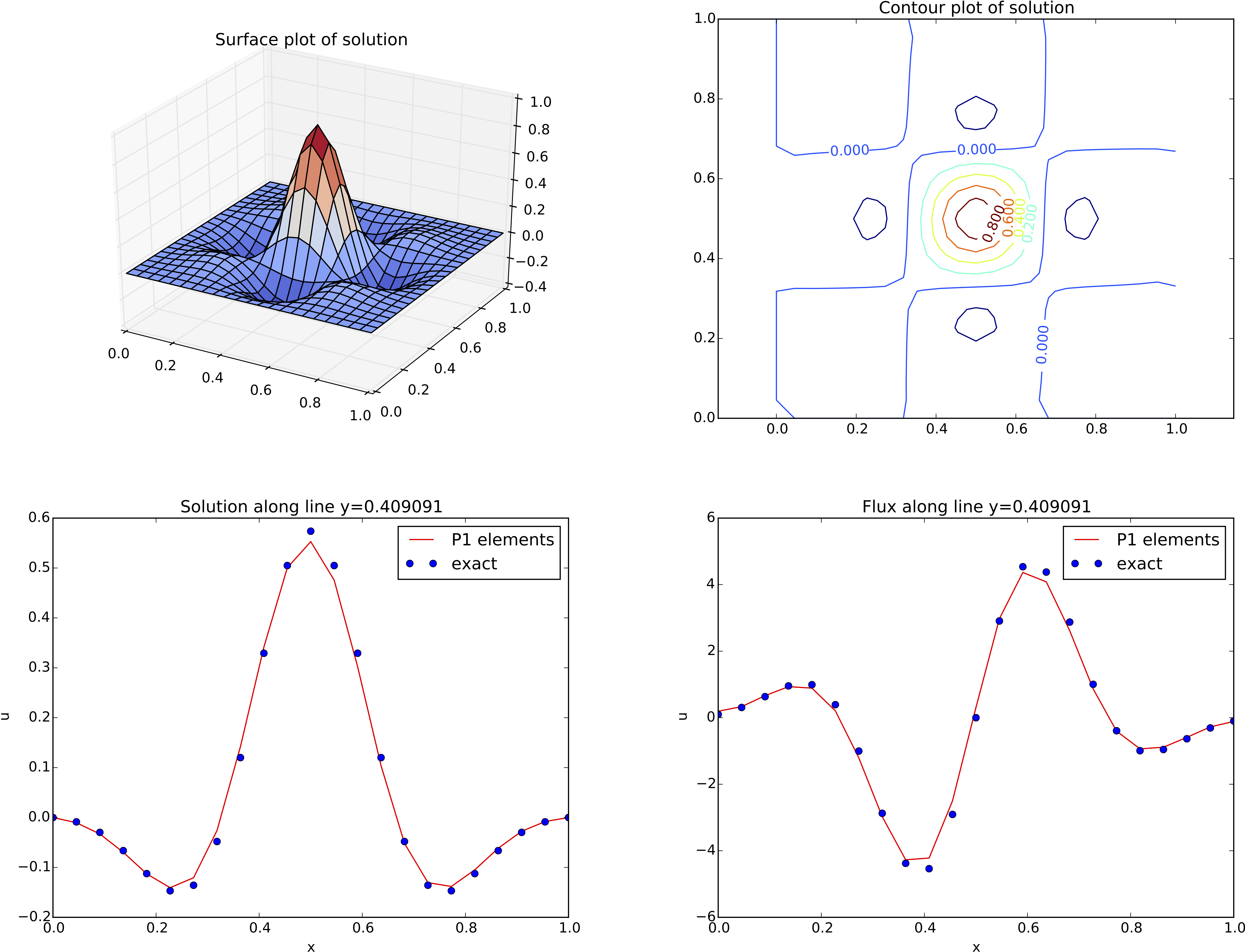
The ability to access a finite element field as structured data is handy in many occasions, e.g., for visualization and data analysis. Using Matplotlib, we can create a surface plot, as shown in Figure 17 (upper left):
import matplotlib.pyplot as plt
from mpl_toolkits.mplot3d import Axes3D  # necessary for 3D plotting
from matplotlib import cm
fig = plt.figure()
ax = fig.gca(projection='3d')
cv = u_box.grid.coorv  # vectorized mesh coordinates
ax.plot_surface(cv[X], cv[Y], u_, cmap=cm.coolwarm,
                rstride=1, cstride=1)
plt.title('Surface plot of solution')
The key issue is to know that the coordinates needed for the surface
plot is in u_box.grid.coorv and that the values are in u_.
Figure 17: Various plots of the solution on a structured mesh.
Making contour plots
A contour plot can also be made by Matplotlib:
fig = plt.figure()
ax = fig.gca()
levels = [1.5, 2.0, 2.5, 3.5]
cs = ax.contour(cv[X], cv[Y], u_, levels=levels)
plt.clabel(cs)  # add labels to contour lines
plt.axis('equal')
plt.title('Contour plot of solution')
The result appears in Figure 17 (upper right).
Making curve plots through the domain
A handy feature of BoxField objects is the ability to give a starting
point in the domain and a direction, and then extract the field and
corresponding coordinates along the nearest line of mesh points. We have
already seen how to interpolate the solution along a line in the mesh, but
with BoxField you can pick out the computational points (vertices) for
examination of these points. Numerical methods often show improved behavior
at such points so this is of interest. For 3D fields
one can also extract data in a plane.
Say we want to plot \( u \) along
the line \( y=0.4 \). The mesh points, x, and the \( u \) values
along this line, u_val, can be extracted by
start = (0, 0.4)
x, u_val, y_fixed, snapped = u_box.gridline(start, direction=X)
The variable snapped is true if the line is snapped onto to nearest
gridline and in that case y_fixed holds the snapped
(altered) \( y \) value. The keyword argument snap is by default True
to avoid interpolation and force snapping.
A comparison of the numerical and exact solution along the line \( y\approx 0.41 \) (snapped from \( y=0.4 \)) is made by the following code:
    # Plot u along a line y = const and compare with exact solution
    start = (0, 0.4)
    x, u_val, y_fixed, snapped = u_box.gridline(start, direction=X)
    u_e_val = [u_D((x_, y_fixed)) for x_ in x]
    plt.figure()
    plt.plot(x, u_val, 'r-')
    plt.plot(x, u_e_val, 'bo')
    plt.legend(['P1 elements', 'exact'], loc='best')
    plt.title('Solution along line y=%g' % y_fixed)
    plt.xlabel('x');  plt.ylabel('u')
See Figure 17 (lower left) for the resulting curve plot.
Making curve plots of the flux
Let us also compare the numerical and exact fluxes \( -\kappa\partial u/\partial x \) along the same line as above:
    # Plot the numerical and exact flux along the same line
    flux_u = flux(u, kappa)
    flux_u_x, flux_u_y = flux_u.split(deepcopy=True)
    flux2_x = flux_u_x if flux_u_x.ufl_element().degree() == 1 \
              else interpolate(flux_x,
                   FunctionSpace(u.function_space().mesh(), 'P', 1))
    flux_u_x_box = FEniCSBoxField(flux_u_x, (nx,ny))
    x, flux_u_val, y_fixed, snapped = \
       flux_u_x_box.gridline(start, direction=X)
    y = y_fixed
    plt.figure()
    plt.plot(x, flux_u_val, 'r-')
    plt.plot(x, flux_u_x_exact(x, y_fixed), 'bo')
    plt.legend(['P1 elements', 'exact'], loc='best')
    plt.title('Flux along line y=%g' % y_fixed)
    plt.xlabel('x');  plt.ylabel('u')
The function flux called at the beginning of the code snippet is
defined in the example program
ft10_poisson_extended.py
and interpolates the flux back into the function space.
Note that Matplotlib is one choice of plotting package. With the unified interface in the SciTools package one can access Matplotlib, Gnuplot, MATLAB, OpenDX, VisIt, and other plotting engines through the same API.
Test problem
The graphics referred to in Figure 17 correspond to
a test problem with prescribed solution \( \uex = H(x)H(y) \), where
$$ H(x) = e^{-16(x-\frac{1}{2})^2}\sin(3\pi x)\tp$$
The corresponding right-hand side \( f \) is obtained by inserting the exact
solution into the PDE and differentiating as before.
Although it is easy to carry out the
differentiation of \( f \) by hand and hardcode the resulting expressions
in an Expression object, a more reliable habit is to use Python's
symbolic computing engine, SymPy, to perform mathematics and
automatically turn formulas into C++ syntax for Expression objects.
A short introduction was given in
the section FEniCS implementation.
We start out with defining the exact solution in sympy:
from sympy import exp, sin, pi  # for use in math formulas
import sympy as sym

H = lambda x: exp(-16*(x-0.5)**2)*sin(3*pi*x)
x, y = sym.symbols('x[0], x[1]')
u = H(x)*H(y)
Turning the expression for u into C or C++ syntax for Expression objects
needs two steps. First we ask for the C code of the expression:
u_code = sym.printing.ccode(u)
Printing u_code gives (the output is here manually broken into two
lines):
-exp(-16*pow(x[0] - 0.5, 2) - 16*pow(x[1] - 0.5, 2))*
sin(3*M_PI*x[0])*sin(3*M_PI*x[1])
The necessary syntax adjustment is replacing
the symbol M_PI for \( \pi \) in C/C++ by pi (or DOLFIN_PI):
u_code = u_code.replace('M_PI', 'pi')
u_b = Expression(u_code, degree=1)
Thereafter, we can progress with the computation of \( f = -\nabla\cdot(\kappa\nabla u) \):
kappa = 1
f = sym.diff(-kappa*sym.diff(u, x), x) + \
    sym.diff(-kappa*sym.diff(u, y), y)
f = sym.simplify(f)
f_code = sym.printing.ccode(f)
f_code = f_code.replace('M_PI', 'pi')
f = Expression(f_code, degree=1)
We also need a Python function for the exact flux \( -\kappa\partial u/\partial x \):
flux_u_x_exact = sym.lambdify([x, y], -kappa*sym.diff(u, x),
                              modules='numpy')
It remains to define kappa = Constant(1) and set nx and ny before calling
solver to compute the finite element solution of this problem.