Deflection of a membrane
Our first FEniCS program for the Poisson equation targeted a simple test problem where we could easily verify the implementation. We now turn our attention to a physically more relevant problem with solutions of somewhat more exciting shape.
We want to compute the deflection \( D(x,y) \) of a two-dimensional, circular membrane of radius \( R \), subject to a load \( p \) over the membrane. The appropriate PDE model is $$ \begin{equation} -T\nabla^2 D = p\quad\hbox{in }\Omega = \{ (x,y)\,\vert\, x^2+y^2\leq R\}\tp \tag{2.14} \end{equation} $$ Here, \( T \) is the tension in the membrane (constant), and \( p \) is the external pressure load. The boundary of the membrane has no deflection, implying \( D=0 \) as a boundary condition. A localized load can be modeled as a Gaussian function: $$ \begin{equation} p(x,y) = {A\over 2\pi\sigma}\exp{\left( - {1\over2}\left( {x-x_0\over\sigma}\right)^2 - {1\over2}\left( {y-y_0\over\sigma}\right)^2 \right)}\, . \tag{2.15} \end{equation} $$ The parameter \( A \) is the amplitude of the pressure, \( (x_0,y_0) \) the localization of the maximum point of the load, and \( \sigma \) the "width" of \( p \). We will take the center \( (x_0,y_0) \) of the pressure to be \( (0, R_0) \) for some \( 0 < R_0 < R \).
Scaling the equation
There are many physical parameters in this problem, and we can benefit from grouping them by means of scaling. Let us introduce dimensionless coordinates \( \bar x = x/R \), \( \bar y = y/R \), and a dimensionless deflection \( w=D/D_c \), where \( D_c \) is a characteristic size of the deflection. Introducing \( \bar R_0=R_0/R \), we obtain $$ -\frac{\partial^2 w}{\partial\bar x^2} -\frac{\partial^2 w}{\partial\bar y^2}= \alpha \exp{\left( - \beta^2(\bar x^2 + (\bar y-\bar R_0)^2)\right)}\hbox{ for } \bar x^2 + \bar y^2 < 1,$$ where $$ \alpha = \frac{R^2A}{2\pi T D_c\sigma},\quad\beta = \frac{R}{\sqrt{2}\sigma}\tp$$ With an appropriate scaling, \( w \) and its derivatives are of size unity, so the left-hand side of the scaled PDE is about unity in size, while the right-hand side has \( \alpha \) as its characteristic size. This suggest choosing \( \alpha \) to be unity, or around unity. We shall in this particular case choose \( \alpha=4 \). (One can also find the analytical solution in scaled coordinates and show that the maximum deflection \( D(0,0) \) is \( D_c \) if we choose \( \alpha=4 \) to determine \( D_c \).) With \( D_c=AR^2/(8\pi\sigma T) \) and dropping the bars we obtain the scaled problem $$ \begin{equation} -\nabla^2w = 4\exp{\left( - \beta^2(x^2 + (y-R_0)^2)\right)}, \tag{2.16} \end{equation} $$ to be solved over the unit disc with \( w=0 \) on the boundary. Now there are only two parameters to vary: the dimensionless extent of the pressure, \( \beta \), and the localization of the pressure peak, \( R_0\in [0,1] \). As \( \beta\rightarrow 0 \), the solution will approach the special case \( w=1-x^2-y^2 \).
Given a computed scaled solution \( w \), the physical deflection can be computed by $$ D = \frac{AR^2}{8\pi\sigma T}w\tp$$
Just a few modifications are necessary to our previous program to solve this new problem.
Defining the mesh
A mesh over the unit disk can be created by the mshr tool in
FEniCS:
from mshr import *
domain = Circle(Point(0, 0), 1)
mesh = generate_mesh(domain, 64)
The Circle shape from mshr takes the center and radius of the
circle as arguments. The second argument to the generate_mesh
function specifies the desired mesh resolution. The cell size will be
(approximately) equal to the diameter of the domain divided by the
resolution.
Defining the load
The right-hand side pressure function
is represented by an Expression object. There
are two physical parameters in the formula for \( f \) that enter the
expression string and these parameters must have their values set
by keyword arguments:
beta = 8
R0 = 0.6
p = Expression('4*exp(-pow(beta, 2)*(pow(x[0], 2) + pow(x[1] - R0, 2)))',
               degree=1, beta=beta, R0=R0)
The coordinates in Expression objects are always an array
x with components x[0], x[1], and x[2], corresponding to
\( x \), \( y \), and \( z \).
Otherwise we are free to introduce names of parameters as long as
these are given default values by keyword arguments. All the
parameters initialized by keyword arguments can at any time have their
values modified. For example, we may set
p.beta = 12
p.R0 = 0.3
Defining the variational problem
The variational problem is the same as in
our first Poisson problem, but we may introduce w instead of u as
primary unknown and p instead of f as right-hand side function:
w = TrialFunction(V)
v = TestFunction(V)
a = dot(grad(w), grad(v))*dx
L = p*v*dx

w = Function(V)
solve(a == L, w, bc)
Plotting the solution
It is of interest to visualize the pressure \( p \) along with the
deflection \( w \) so that we may examine the membrane's response to the
pressure. We must then transform the formula (Expression) to a
finite element function (Function). The most natural approach is to
construct a finite element function whose degrees of freedom are
calculated from \( p \). That is, we interpolate \( p \) to the function space
\( V \):
p = interpolate(p, V)
Note that the assignment to p destroys the previous Expression
object p, so if it is of interest to still have access to this
object, another name must be used for the Function object returned
by interpolate. The two functions w and p may be plotted
using the built-in plot command:
plot(w, title='Deflection')
plot(p, title='Load')
As before, we also export the solutions in VTK format for visualization in ParaView:
vtkfile_w = File('poisson_membrane/deflection.pvd')
vtkfile_w << w
vtkfile_p = File('poisson_membrane/load.pvd')
vtkfile_p << p
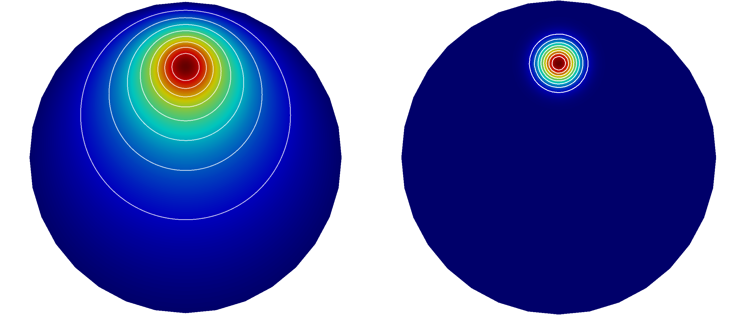
Figure 3 shows a visualization
of the deflection w and the load p created with ParaView.
Figure 3: Plot of the deflection (left) and load (right) for the membrane problem created using ParaView. The plot uses 10 equispaced isolines for the solution values and the optional jet colormap.
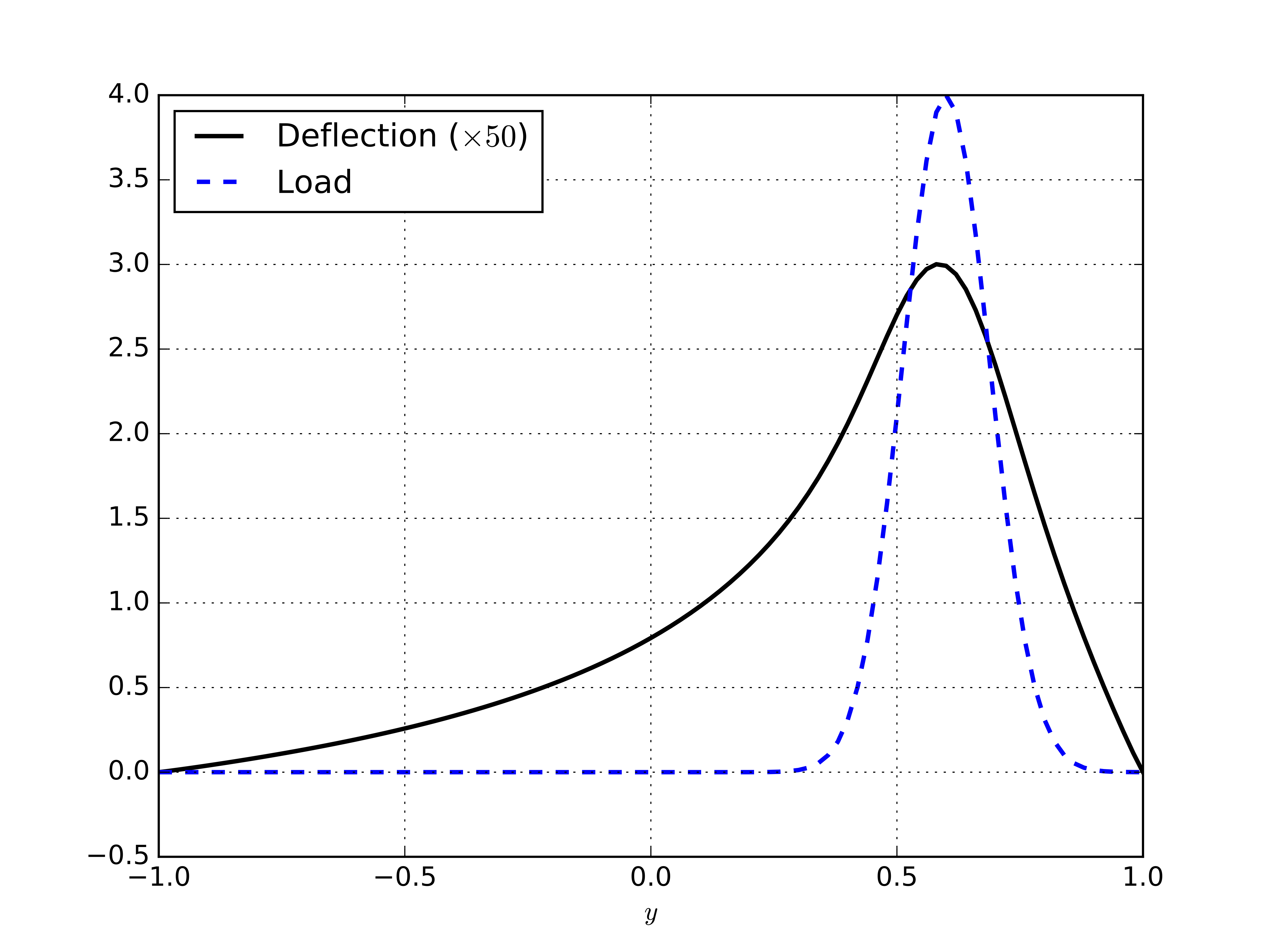
Making curve plots through the domain
Another way to compare the deflection and the load is to make a curve plot
along the line \( x=0 \). This is just a matter of defining a set of points
along the \( y \)-axis and evaluating the finite element functions w and p
at these points:
# Curve plot along x = 0 comparing p and w
import numpy as np
import matplotlib.pyplot as plt
tol = 0.001  # avoid hitting points outside the domain
y = np.linspace(-1 + tol, 1 - tol, 101)
points = [(0, y_) for y_ in y]  # 2D points
w_line = np.array([w(point) for point in points])
p_line = np.array([p(point) for point in points])
plt.plot(y, 50*w_line, 'k', linewidth=2)  # magnify w
plt.plot(y, p_line, 'b--', linewidth=2)
plt.grid(True)
plt.xlabel('$y$')
plt.legend(['Deflection ($\\times 50$)', 'Load'], loc='upper left')
plt.savefig('poisson_membrane/curves.pdf')
plt.savefig('poisson_membrane/curves.png')
This example program can be found in the file ft02_poisson_membrane.py.
The resulting curve plot is shown in Figure 4. The localized input (\( p \)) is heavily damped and smoothed in the output (\( w \)). This reflects a typical property of the Poisson equation.
Figure 4: Plot of the deflection and load for the membrane problem created using Matplotlib and sampling of the two functions along the \( y \)-axsis.