The equations of linear elasticity

Analysis of structures is one of the major activities of modern engineering, which likely makes the PDE modeling the deformation of elastic bodies the most popular PDE in the world. It takes just one page of code to solve the equations of 2D or 3D elasticity in FEniCS, and the details follow below.

PDE problem

The equations governing small elastic deformations of a body $ \Omega $ can be written as $$ \begin{align} -\nabla\cdot\sigma &= f\hbox{ in }\Omega, \tag{3.20}\\ \sigma &= \lambda\,\hbox{tr}\,(\varepsilon) I + 2\mu\varepsilon, \tag{3.21}\\ \varepsilon &= \frac{1}{2}\left(\nabla u + (\nabla u)^{\top}\right), \tag{3.22} \end{align} $$ where $ \sigma $ is the stress tensor, $ f $ is the body force per unit volume, $ \lambda $ and $ \mu $ are $ \text{Lam\'e's} $ elasticity parameters for the material in $ \Omega $, $ I $ is the identity tensor, $ \mathrm{tr} $ is the trace operator on a tensor, $ \varepsilon $ is the symmetric strain-rate tensor (symmetric gradient), and $ u $ is the displacement vector field. We have here assumed isotropic elastic conditions.

We combine (3.21) and (3.22) to obtain $$ \begin{equation} \sigma = \lambda(\nabla\cdot u)I + \mu(\nabla u + (\nabla u)^{\top})\tp \tag{3.23} \end{equation} $$ Note that (3.20)--(3.22) can easily be transformed to a single vector PDE for $ u $, which is the governing PDE for the unknown $ u $ (Navier's equation). In the derivation of the variational formulation, however, it is convenient to keep the equations split as above.

Variational formulation

The variational formulation of (3.20)--(3.22) consists of forming the inner product of (3.20) and a vector test function $ v\in \hat{V} $, where $ \hat{V} $ is a vector-valued test function space, and integrating over the domain $ \Omega $: $$ -\int_\Omega (\nabla\cdot\sigma) \cdot v \dx = \int_\Omega f\cdot v\dx\tp$$ Since $ \nabla\cdot\sigma $ contains second-order derivatives of the primary unknown $ u $, we integrate this term by parts: $$ -\int_\Omega (\nabla\cdot\sigma) \cdot v \dx = \int_\Omega \sigma : \nabla v\dx - \int_{\partial\Omega} (\sigma\cdot n)\cdot v \ds,$$ where the colon operator is the inner product between tensors (summed pairwise product of all elements), and $ n $ is the outward unit normal at the boundary. The quantity $ \sigma\cdot n $ is known as the traction or stress vector at the boundary, and is often prescribed as a boundary condition. We here assume that it is prescribed on a part $ \partial\Omega_T $ of the boundary as $ \sigma\cdot n = T $. On the remaining part of the boundary, we assume that the value of the displacement is given as a Dirichlet condition. We thus obtain $$ \int_\Omega \sigma : \nabla v \dx = \int_\Omega f\cdot v \dx + \int_{\partial\Omega_T} T\cdot v\ds\tp$$ Inserting the expression (3.23) for $ \sigma $ gives the variational form with $ u $ as unknown. Note that the boundary integral on the remaining part $ \partial\Omega\setminus\partial\Omega_T $ vanishes due to the Dirichlet condition.

We can now summarize the variational formulation as: find $ u\in V $ such that $$ \begin{equation} a(u,v) = L(v)\quad\forall v\in\hat{V}, \tag{3.24} \end{equation} $$ where $$ \begin{align} a(u,v) &= \int_\Omega\sigma(u) :\nabla v \dx, \tag{3.25} \\ \sigma(u) &= \lambda(\nabla\cdot u)I + \mu(\nabla u + (\nabla u)^{\top}), \tag{3.26}\\ L(v) &= \int_\Omega f\cdot v\dx + \int_{\partial\Omega_T} T\cdot v\ds\tp \tag{3.27} \end{align} $$

One can show that the inner product of a symmetric tensor $ A $ and an anti-symmetric tensor $ B $ vanishes. If we express $ \nabla v $ as a sum of its symmetric and anti-symmetric parts, only the symmetric part will survive in the product $ \sigma :\nabla v $ since $ \sigma $ is a symmetric tensor. Thus replacing $ \nabla u $ by the symmetric gradient $ \epsilon(u) $ gives rise to the slightly different variational form $$ \begin{equation} a(u,v) = \int_\Omega\sigma(u) :\varepsilon(v) \dx, \tag{3.28} \end{equation} $$ where $ \varepsilon(v) $ is the symmetric part of $ \nabla v $: $$ \varepsilon(v) = \frac{1}{2}\left(\nabla v + (\nabla v)^{\top}\right)\tp$$ The formulation (3.28) is what naturally arises from minimization of elastic potential energy and is a more popular formulation than (3.25).

FEniCS implementation

Test problem

As a test example, we will model a clamped beam deformed under its own weight in 3D. This can be modeled by setting the right-hand side body force per unit volume to $ f=(0,0,-\varrho g) $ with $ \varrho $ the density of the beam and $ g $ the acceleration of gravity. The beam is box-shaped with length $ L $ and has a square cross section of width $ W $. We set $ u=\ub = (0,0,0) $ at the clamped end, $ x=0 $. The rest of the boundary is traction free; that is, we set $ T = 0 $.

FEniCS implementation

We first list the code and then comment upon the new constructions compared to the previous examples we have seen.

from fenics import *

# Scaled variables
L = 1; W = 0.2
mu = 1
rho = 1
delta = W/L
gamma = 0.4*delta**2
beta = 1.25
lambda_ = beta
g = gamma

# Create mesh and define function space
mesh = BoxMesh(Point(0, 0, 0), Point(L, W, W), 10, 3, 3)
V = VectorFunctionSpace(mesh, 'P', 1)

# Define boundary condition
tol = 1E-14

def clamped_boundary(x, on_boundary):
    return on_boundary and x[0] < tol

bc = DirichletBC(V, Constant((0, 0, 0)), clamped_boundary)

# Define strain and stress

def epsilon(u):
    return 0.5*(nabla_grad(u) + nabla_grad(u).T)
    #return sym(nabla_grad(u))

def sigma(u):
    return lambda_*nabla_div(u)*Identity(d) + 2*mu*epsilon(u)

# Define variational problem
u = TrialFunction(V)
d = u.geometric_dimension()  # space dimension
v = TestFunction(V)
f = Constant((0, 0, -rho*g))
T = Constant((0, 0, 0))
a = inner(sigma(u), epsilon(v))*dx
L = dot(f, v)*dx + dot(T, v)*ds

# Compute solution
u = Function(V)
solve(a == L, u, bc)

# Plot solution
plot(u, title='Displacement', mode='displacement')

# Plot stress
s = sigma(u) - (1./3)*tr(sigma(u))*Identity(d)  # deviatoric stress
von_Mises = sqrt(3./2*inner(s, s))
V = FunctionSpace(mesh, 'P', 1)
von_Mises = project(von_Mises, V)
plot(von_Mises, title='Stress intensity')

# Compute magnitude of displacement
u_magnitude = sqrt(dot(u, u))
u_magnitude = project(u_magnitude, V)
plot(u_magnitude, 'Displacement magnitude')
print('min/max u:',
      u_magnitude.vector().array().min(),
      u_magnitude.vector().array().max())

This example program can be found in the file ft06_elasticity.py.

Vector function spaces

The primary unknown is now a vector field $ u $ and not a scalar field, so we need to work with a vector function space:

V = VectorFunctionSpace(mesh, 'P', 1)

With u = Function(V) we get u as a vector-valued finite element function with three components for this 3D problem.

Constant vectors

For the boundary condition $ u=(0, 0, 0) $, we must set a vector value to zero, not just a scalar. Such a vector constant is specified as Constant((0, 0, 0)) in FEniCS. The corresponding 2D code would use Constant((0, 0)). Later in the code, we also need f as a vector and specify it as Constant((0, 0, rho*g)).

`nabla_grad`

The gradient and divergence operators now have a prefix nabla_. This is strictly not necessary in the present problem, but recommended in general for vector PDEs arising from continuum mechanics, if you interpret $ \nabla $ as a vector in the PDE notation; see the box about nabla_grad in the section Variational formulation.

Stress computation

As soon as the displacement u is computed, we can compute various stress measures. We will compute the von Mises stress defined as $ \sigma_M = \sqrt{\frac{3}{2}s:s} $ where $ s $ is the deviatoric stress tensor $$ s = \sigma - \frac{1}{3}\mathrm{tr}\,(\sigma)\,I\tp$$ There is a one-to-one mapping between these formulas and the FEniCS code:

s = sigma(u) - (1./3)*tr(sigma(u))*Identity(d)
von_Mises = sqrt(3./2*inner(s, s))

The von_Mises variable is now an expression that must be projected to a finite element space before we can visualize it:

V = FunctionSpace(mesh, 'P', 1)
von_Mises = project(von_Mises, V)
plot(von_Mises, title='Stress intensity')

Scaling

It is often advantageous to scale a problem as it reduces the need for setting physical parameters, and one obtains dimensionsless numbers that reflect the competition of parameters and physical effects. We develop the code for the original model with dimensions, and run the scaled problem by tweaking parameters appropriately. Scaling reduces the number of active parameters from 6 to 2 for the present application.

In Navier's equation for $ u $, arising from inserting (3.21) and (3.22) into (3.20), $$ -(\lambda + \mu)\nabla(\nabla\cdot u) - \mu\nabla^2 u = f,$$ we insert coordinates made dimensionless by $ L $, and $ \bar u=u/U $, which results in the dimensionless governing equation $$ -\beta\bar\nabla(\bar\nabla\cdot \bar u) - \bar\nabla^2 \bar u = \bar f,\quad \bar f = (0,0,\gamma),$$ where $ \beta = 1 + \lambda/\mu $ is a dimensionless elasticity parameter and where $$ \gamma = \frac{\varrho gL^2}{\mu U}$$ is a dimensionless variable reflecting the ratio of the load $ \varrho g $ and the shear stress term $ \mu\nabla^2 u\sim \mu U/L^2 $ in the PDE.

One option for the scaling is to chose $ U $ such that $ \gamma $ is of unit size ($ U = \varrho gL^2/\mu $). However, in elasticity, this leads to displacements of the size of the geometry, which makes plots look very strange. We therefore want the characteristic displacement to be a small fraction of the characteristic length of the geometry. This can be achieved by choosing $ U $ equal to the maximum deflection of a clamped beam, for which there actually exists a formula: $ U = \frac{3}{2}\varrho gL^2\delta^2/E $, where $ \delta = L/W $ is a parameter reflecting how slender the beam is, and $ E $ is the modulus of elasticity. Thus, the dimensionless parameter $ \delta $ is very important in the problem (as expected, since $ \delta\gg 1 $ is what gives beam theory!). Taking $ E $ to be of the same order as $ \mu $, which is the case for many materials, we realize that $ \gamma \sim \delta^{-2} $ is an appropriate choice. Experimenting with the code to find a displacement that "looks right" in plots of the deformed geometry, points to $ \gamma = 0.4\delta^{-2} $ as our final choice of $ \gamma $.

The simulation code implements the problem with dimensions and physical parameters $ \lambda $, $ \mu $, $ \varrho $, $ g $, $ L $, and $ W $. However, we can easily reuse this code for a scaled problem: just set $ \mu = \varrho = L = 1 $, $ W $ as $ W/L $ ($ \delta^{-1} $), $ g=\gamma $, and $ \lambda=\beta $.

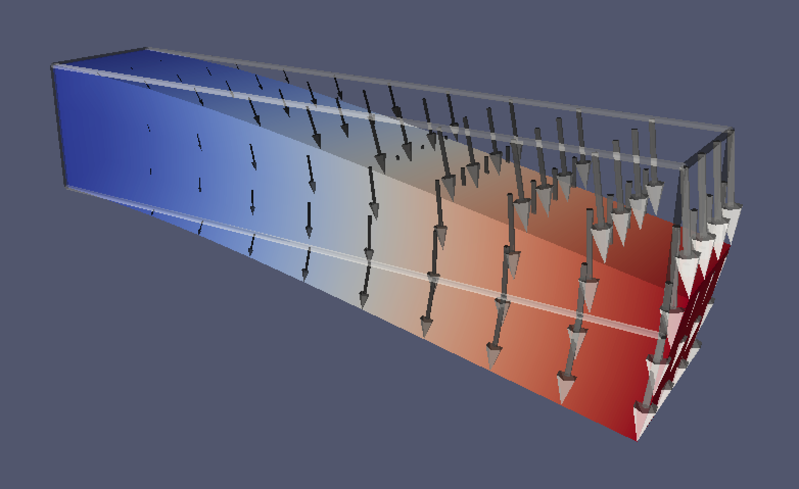
Figure 6: Plot of gravity-induced deflection in a clamped beam for the elasticity problem.