Degrees of freedom and function evaluation
Examining the degrees of freedom
We have seen before how to grab the degrees of freedom array from a
finite element function u:
nodal_values = u.vector().array()
For a finite element function from a standard continuous piecewise linear function space (\( \mathsf{P}_1 \) Lagrange elements), these values will be the same as the values we get by the following statement:
vertex_values = u.compute_vertex_values(mesh)
Both nodal_values and vertex_values will be numpy arrays and
they will be of the same length and contain the same values (for
\( \mathsf{P}_1 \) elements), but with possibly different ordering. The
array vertex_values will have the same ordering as the vertices of
the mesh, while nodal_values will be ordered in a way that (nearly)
minimizes the bandwidth of the system matrix and thus improves the
efficiency of linear solvers.
A fundamental question is: what are the
coordinates of the vertex whose value is nodal_values[i]? To answer this
question, we need to understand how to get our hands on the
coordinates, and in particular, the numbering of degrees of freedom
and the numbering of vertices in the mesh.
The function mesh.coordinates returns the coordinates of the
vertices as a numpy array with shape \( (M,d) \), \( M \) being the number
of vertices in the mesh and \( d \) being the number of space dimensions:
>>> from fenics import *
>>> mesh = UnitSquareMesh(2, 2)
>>> coordinates = mesh.coordinates()
>>> coordinates
array([[ 0. ,  0. ],
       [ 0.5,  0. ],
       [ 1. ,  0. ],
       [ 0. ,  0.5],
       [ 0.5,  0.5],
       [ 1. ,  0.5],
       [ 0. ,  1. ],
       [ 0.5,  1. ],
       [ 1. ,  1. ]])
We see from this output that for this particular mesh, the vertices are first numbered along \( y=0 \) with increasing \( x \) coordinate, then along \( y=0.5 \), and so on.
Next we compute a function u on this mesh. Let's take \( u=x+y \):
>>> V = FunctionSpace(mesh, 'P', 1)
>>> u = interpolate(Expression('x[0] + x[1]', degree=1), V)
>>> plot(u, interactive=True)
>>> nodal_values = u.vector().array()
>>> nodal_values
array([ 1. ,  0.5,  1.5,  0. ,  1. ,  2. ,  0.5,  1.5,  1. ])
We observe that nodal_values[0] is not the value of \( x+y \) at
vertex number 0, since this vertex has coordinates \( x=y=0 \). The
numbering of the nodal values (degrees of freedom) \( U_1,\ldots,U_{N} \)
is obviously not the same as the numbering of the vertices.
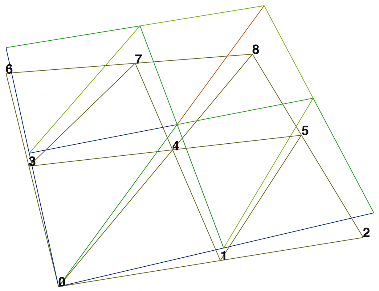
The vertex numbering may be examined by using the FEniCS plot
command. To do this, plot the function u, press w to turn on
wireframe instead of a fully colored surface, m to show the mesh,
and then v to show the numbering of the vertices.
Let's instead examine the values by calling
u.compute_vertex_values:
>>> vertex_values = u.compute_vertex_values()
>>> for i, x in enumerate(coordinates):
...     print('vertex %d: vertex_values[%d] = %g\tu(%s) = %g' %
...           (i, i, vertex_values[i], x, u(x)))
vertex 0: vertex_values[0] = 0          u([ 0.  0.]) = 8.46545e-16
vertex 1: vertex_values[1] = 0.5        u([ 0.5  0. ]) = 0.5
vertex 2: vertex_values[2] = 1          u([ 1.  0.]) = 1
vertex 3: vertex_values[3] = 0.5        u([ 0.   0.5]) = 0.5
vertex 4: vertex_values[4] = 1          u([ 0.5  0.5]) = 1
vertex 5: vertex_values[5] = 1.5        u([ 1.   0.5]) = 1.5
vertex 6: vertex_values[6] = 1          u([ 0.  1.]) = 1
vertex 7: vertex_values[7] = 1.5        u([ 0.5  1. ]) = 1.5
vertex 8: vertex_values[8] = 2          u([ 1.  1.]) = 2
We can ask FEniCS to give us the mapping from vertices to degrees of freedom for a certain function space \( V \):
v2d = vertex_to_dof_map(V)
Now, nodal_values[v2d[i]] will give us the value of the degree of
freedom
corresponding to vertex i (v2d[i]). In particular, nodal_values[v2d]
is an array with all the elements in the same (vertex numbered) order
as coordinates. The inverse map, from degrees of freedom number to
vertex number is given by dof_to_vertex_map(V). This means that
we may call
coordinates[dof_to_vertex_map(V)] to get an array of all the
coordinates in the same order as the degrees of freedom. Note that
these mappings are only available in FEniCS for \( \mathsf{P}_1 \) elements.
For Lagrange elements of degree larger than 1, there are degrees of
freedom (nodes) that do not correspond to vertices. For these
elements, we may get the vertex values by calling
u.compute_vertex_values(mesh), and we can get the degrees of freedom
by the call u.vector().array(). To get the coordinates associated
with all degrees of freedom, we need to iterate over the elements of
the mesh and ask FEniCS to return the coordinates and dofs associated
with each element (cell). This information is stored in the
FiniteElement and DofMap object of a FunctionSpace. The
following code illustrates how to iterate over all elements of a mesh
and print the coordinates and degrees of freedom associated with the
element.
element = V.element()
dofmap = V.dofmap()
for cell in cells(mesh):
    print(element.tabulate_dof_coordinates(cell))
    print(dofmap.cell_dofs(cell.index()))
Setting the degrees of freedom
We have seen how to extract the nodal values in a numpy array.
If desired, we can adjust the nodal values too. Say we want to
normalize the solution such that \( \max_j |U_j| = 1 \). Then we
must divide all \( U_j \) values
by \( \max_j |U_j| \). The following function performs the task:
def normalize_solution(u):
    "Normalize u: return u divided by max(u)"
    u_array = u.vector().array()
    u_max = np.max(np.abs(u_array))
    u_array /= u_max
    u.vector()[:] = u_array
    #u.vector().set_local(u_array)  # alternative
    return u
When using Lagrange elements, this (approximately) ensures that the maximum value of the function \( u \) is \( 1 \).
The /= operator implies an
in-place modification of the object on the left-hand side: all
elements of the array nodal_values are divided by the value u_max.
Alternatively, we could do nodal_values = nodal_values / u_max, which
implies creating a new array on the right-hand side and assigning this
array to the name nodal_values.
u.vector().array() returns a copy of the data in
u.vector(). One must therefore never perform assignments like
u.vector.array()[:] = ..., but instead extract the numpy array
(i.e., a copy), manipulate it, and insert it back with u.vector()[:]
= or use u.set_local(...).
Function evaluation
A FEniCS Function object is uniquely defined in the interior
of each cell of the finite element mesh. For continuous (Lagrange)
function spaces, the function values are also uniquely defined on
cell boundaries. A Function object u can be evaluated by simply
calling
u(x)
where x is either a Point or a Python tuple of the correct space
dimension. When a Function is evaluated, FEniCS must first find
which cell of the mesh that contains the given point (if any), and
then evaluate a linear combination of basis functions at the given
point inside the cell in question. FEniCS uses efficient data
structures (bounding box trees) to quickly find the point, but
building the tree is a relatively expensive operation so the cost of
evaluating a Function at a single point is costly. Repeated
evaluation will reuse the computed data structures and thus be
relatively less expensive.
Function object u can be evaluated in various ways:
-
u(x)for an arbitrary pointx -
u.vector().array()[i]for degree of freedom numberi -
u.compute_vertex_values()[i]at vertex numberi
To demonstrate the use of point evaluation of Function objects, we
print the value of the computed finite element solution u for the
Poisson problem at the center point of the domain and compare it with
the exact solution:
center = (0.5, 0.5)
error = u_D(center) - u(center)
print('Error at %s: %g' % (center, error))
For a \( 2\times(3\times 3) \) mesh, the output from the previous snippet becomes
Error at (0.5, 0.5): -0.0833333
The discrepancy is due to the fact that the center point is not a node
in this particular mesh, but a point in the interior of a cell, and
u varies linearly over the cell while u_D is a quadratic
function. When the center point is a node, as in a \( 2\times(2\times
2) \) or \( 2\times(4\times 4) \) mesh, the error is of the order
\( 10^{-15} \).