Fundamentals: Solving the Poisson equation

The goal of this chapter is to show how the Poisson equation, the most basic of all PDEs, can be quickly solved with a few lines of FEniCS code. We introduce the most fundamental FEniCS objects such as Mesh, Function, FunctionSpace, TrialFunction, and TestFunction, and learn how to write a basic PDE solver, including how to formulate the mathematical variational problem, apply boundary conditions, call the FEniCS solver, and plot the solution.

Mathematical problem formulation

Many books on programming languages start with a "Hello, World!" program. Readers are curious to know how fundamental tasks are expressed in the language, and printing a text to the screen can be such a task. In the world of finite element methods for PDEs, the most fundamental task must be to solve the Poisson equation. Our counterpart to the classical "Hello, World!" program therefore solves the following boundary-value problem: $$ \begin{alignat}{2} - \nabla^2 u(\x) &= f(\x),\quad &&\x\mbox{ in } \Omega, \tag{2.1}\\ u(\x) &= \ub(\x),\quad &&\x\mbox{ on } \partial \Omega\tp \tag{2.2} \end{alignat} $$ Here, $ u = u(\x) $ is the unknown function, $ f = f(\x) $ is a prescribed function, $ \nabla^2 $ is the Laplace operator (often written as $ \Delta $), $ \Omega $ is the spatial domain, and $ \partial\Omega $ is the boundary of $ \Omega $. The Poisson problem, including both the PDE $ -\nabla^2 u = f $ and the boundary condition $ u = \ub $ on $ \partial \Omega $, is an example of a boundary-value problem, which must be precisely stated before it makes sense to start solving it with FEniCS.

In two space dimensions with coordinates $ x $ and $ y $, we can write out the Poisson equation as $$ \begin{equation} - {\partial^2 u\over\partial x^2} - {\partial^2 u\over\partial y^2} = f(x,y)\tp \tag{2.3} \end{equation} $$ The unknown $ u $ is now a function of two variables, $ u = u(x,y) $, defined over a two-dimensional domain $ \Omega $.

The Poisson equation arises in numerous physical contexts, including heat conduction, electrostatics, diffusion of substances, twisting of elastic rods, inviscid fluid flow, and water waves. Moreover, the equation appears in numerical splitting strategies for more complicated systems of PDEs, in particular the Navier–Stokes equations.

Solving a boundary-value problem such as the Poisson equation in FEniCS consists of the following steps:

Identify the computational domain ($ \Omega $), the PDE, its boundary conditions, and source terms ($ f $).
Reformulate the PDE as a finite element variational problem.
Write a Python program which defines the computational domain, the variational problem, the boundary conditions, and source terms, using the corresponding FEniCS abstractions.
Call FEniCS to solve the boundary-value problem and, optionally, extend the program to compute derived quantities such as fluxes and averages, and visualize the results.

We shall now go through steps 2–4 in detail. The key feature of FEniCS is that steps 3 and 4 result in fairly short code, while a similar program in most other software frameworks for PDEs require much more code and technically difficult programming.

What makes FEniCS attractive? Although many software frameworks have a really elegant "Hello, World!" example for the Poisson equation, FEniCS is to our knowledge the only framework where the code stays compact and nice, very close to the mathematical formulation, even when the mathematical and algorithmic complexity increases and when moving from a laptop to a high-performance compute server (cluster).

Finite element variational formulation

FEniCS is based on the finite element method, which is a general and efficient mathematical machinery for the numerical solution of PDEs. The starting point for the finite element methods is a PDE expressed in variational form. Readers who are not familiar with variational problems will get a very brief introduction to the topic in this tutorial, but reading a proper book on the finite element method in addition is encouraged. The section The finite element method contains a list of recommended books. Experience shows that you can work with FEniCS as a tool to solve PDEs even without thorough knowledge of the finite element method, as long as you get somebody to help you with formulating the PDE as a variational problem.

The basic recipe for turning a PDE into a variational problem is to multiply the PDE by a function $ v $, integrate the resulting equation over the domain $ \Omega $, and perform integration by parts of terms with second-order derivatives. The function $ v $ which multiplies the PDE is called a test function. The unknown function $ u $ to be approximated is referred to as a trial function. The terms trial and test functions are used in FEniCS programs too. The trial and test functions belong to certain so-called function spaces that specify the properties of the functions.

In the present case, we first multiply the Poisson equation by the test function $ v $ and integrate over $ \Omega $: $$ \begin{equation} \tag{2.4} -\int_\Omega (\nabla^2 u)v \dx = \int_\Omega fv \dx\tp \end{equation} $$ We here let $ \dx $ denote the differential element for integration over the domain $ \Omega $. We will later let $ \ds $ denote the differential element for integration over the boundary of $ \Omega $.

A common rule when we derive variational formulations is that we try to keep the order of the derivatives of $ u $ and $ v $ as small as possible. Here, we have a second-order spatial derivative of $ u $, which can be transformed to a first-derivative of $ u $ and $ v $ by applying the technique of integration by parts. The formula reads $$ \begin{equation} \tag{2.5} -\int_\Omega (\nabla^2 u)v \dx = \int_\Omega\nabla u\cdot\nabla v \dx - \int_{\partial\Omega}{\partial u\over \partial n}v \ds , \end{equation} $$ where $ \frac{\partial u}{\partial n} = \nabla u \cdot n $ is the derivative of $ u $ in the outward normal direction $ n $ on the boundary.

Another feature of variational formulations is that the test function $ v $ is required to vanish on the parts of the boundary where the solution $ u $ is known (the book [14] explains in detail why this requirement is necessary). In the present problem, this means that $ v=0 $ on the whole boundary $ \partial\Omega $. The second term on the right-hand side of (2.5) therefore vanishes. From (2.4) and (2.5) it follows that $$ \begin{equation} \int_\Omega\nabla u\cdot\nabla v \dx = \int_\Omega fv \dx\tp \tag{2.6} \end{equation} $$ If we require that this equation holds for all test functions $ v $ in some suitable space $ \hat V $, the so-called test space, we obtain a well-defined mathematical problem that uniquely determines the solution $ u $ which lies in some (possibly different) function space $ V $, the so-called trial space. We refer to (2.6) as the weak form or variational form of the original boundary-value problem (2.1)--(2.2).

The proper statement of our variational problem now goes as follows: find $ u \in V $ such that $$ \begin{equation} \tag{2.7} \int_{\Omega} \nabla u \cdot \nabla v \dx = \int_{\Omega} fv \dx \quad \forall v \in \hat{V}\tp \end{equation} $$ The trial and test spaces $ V $ and $ \hat V $ are in the present problem defined as $$ \begin{align*} V &= \{v \in H^1(\Omega) : v = \ub \mbox{ on } \partial\Omega\}, \\ \hat{V} &= \{v \in H^1(\Omega) : v = 0 \mbox{ on } \partial\Omega\}\tp \end{align*} $$ In short, $ H^1(\Omega) $ is the mathematically well-known Sobolev space containing functions $ v $ such that $ v^2 $ and $ |\nabla v|^2 $ have finite integrals over $ \Omega $ (essentially meaning that the functions are continuous). The solution of the underlying PDE must lie in a function space where the derivatives are also continuous, but the Sobolev space $ H^1(\Omega) $ allows functions with discontinuous derivatives. This weaker continuity requirement of $ u $ in the variational statement (2.7), as a result of the integration by parts, has great practical consequences when it comes to constructing finite element function spaces. In particular, it allows the use of piecewise polynomial function spaces; i.e., function spaces constructed by stitching together polynomial functions on simple domains such as intervals, triangles, or tetrahedrons.

The variational problem (2.7) is a continuous problem: it defines the solution $ u $ in the infinite-dimensional function space $ V $. The finite element method for the Poisson equation finds an approximate solution of the variational problem (2.7) by replacing the infinite-dimensional function spaces $ V $ and $ \hat{V} $ by discrete (finite-dimensional) trial and test spaces $ V_h\subset{V} $ and $ \hat{V}_h\subset\hat{V} $. The discrete variational problem reads: find $ u_h \in V_h \subset V $ such that $$ \begin{equation} \tag{2.8} \int_{\Omega} \nabla u_h \cdot \nabla v \dx = \int_{\Omega} fv \dx \quad \forall v \in \hat{V}_h \subset \hat{V}\tp \end{equation} $$

This variational problem, together with a suitable definition of the function spaces $ V_h $ and $ \hat{V}_h $, uniquely define our approximate numerical solution of Poisson's equation (2.1). Note that the boundary conditions are encoded as part of the trial and test spaces. The mathematical framework may seem complicated at first glance, but the good news is that the finite element variational problem (2.8) looks the same as the continuous variational problem (2.7), and FEniCS can automatically solve variational problems like (2.8)!

What we mean by the notation $ u $ and $ V $. The mathematics literature on variational problems writes $ u_h $ for the solution of the discrete problem and $ u $ for the solution of the continuous problem. To obtain (almost) a one-to-one relationship between the mathematical formulation of a problem and the corresponding FEniCS program, we shall drop the subscript $ _h $ and use $ u $ for the solution of the discrete problem. We will use $ \uex $ for the exact solution of the continuous problem, if we need to explicitly distinguish between the two. Similarly, we will let $ V $ denote the discrete finite element function space in which we seek our solution.

Abstract finite element variational formulation

It turns out to be convenient to introduce the following canonical notation for variational problems: find $ u\in V $ such that $$ \begin{equation} a(u, v) = L(v) \quad \forall v \in \hat{V}. \tag{2.9} \end{equation} $$ For the Poisson equation, we have: $$ \begin{align} a(u, v) &= \int_{\Omega} \nabla u \cdot \nabla v \dx, \tag{2.10}\\ L(v) &= \int_{\Omega} fv \dx\tp \tag{2.11} \end{align} $$ From the mathematics literature, $ a(u,v) $ is known as a bilinear form and $ L(v) $ as a linear form. We shall, in every linear problem we solve, identify the terms with the unknown $ u $ and collect them in $ a(u,v) $, and similarly collect all terms with only known functions in $ L(v) $. The formulas for $ a $ and $ L $ can then be expressed directly in our FEniCS programs.

To solve a linear PDE in FEniCS, such as the Poisson equation, a user thus needs to perform only two steps:

Choose the finite element spaces $ V $ and $ \hat V $ by specifying the domain (the mesh) and the type of function space (polynomial degree and type).
Express the PDE as a (discrete) variational problem: find $ u\in V $ such that $ a(u,v) = L(v) $ for all $ v\in \hat{V} $.

Choosing a test problem

The Poisson problem (2.1)--(2.2) has so far featured a general domain $ \Omega $ and general functions $ \ub $ for the boundary conditions and $ f $ for the right-hand side. For our first implementation we will need to make specific choices for $ \Omega $, $ \ub $, and $ f $. It will be wise to construct a problem with a known analytical solution so that we can easily check that the computed solution is correct. Solutions that are lower-order polynomials are primary candidates. Standard finite element function spaces of degree $ r $ will exactly reproduce polynomials of degree $ r $. And piecewise linear elements ($ r=1 $) are able to exactly reproduce a quadratic polynomial on a uniformly partitioned mesh. This important result can be used to verify our implementation. We just manufacture some quadratic function in 2D as the exact solution, say $$ \begin{equation} \tag{2.12} \uex(x,y) = 1 +x^2 + 2y^2\tp \end{equation} $$ By inserting (2.12) into the Poisson equation (2.1), we find that $ \uex(x,y) $ is a solution if $$ f(x,y) = -6,\quad \ub(x,y)=\uex(x,y)=1 + x^2 + 2y^2,$$ regardless of the shape of the domain as long as $ \uex $ is prescribed along the boundary. We choose here, for simplicity, the domain to be the unit square, $$ \Omega = [0,1]\times [0,1] \tp$$ This simple but very powerful method for constructing test problems is called the method of manufactured solutions: pick a simple expression for the exact solution, plug it into the equation to obtain the right-hand side (source term $ f $), then solve the equation with this right-hand side and using the exact solution as a boundary condition, and try to reproduce the exact solution.

Tip: Try to verify your code with exact numerical solutions! A common approach to testing the implementation of a numerical method is to compare the numerical solution with an exact analytical solution of the test problem and conclude that the program works if the error is "small enough". Unfortunately, it is impossible to tell if an error of size $ 10^{-5} $ on a $ 20\times 20 $ mesh of linear elements is the expected (in)accuracy of the numerical approximation or if the error also contains the effect of a bug in the code. All we usually know about the numerical error is its asymptotic properties, for instance that it is proportional to $ h^2 $ if $ h $ is the size of a cell in the mesh. Then we compare the error on meshes with different $ h $-values to see if the asymptotic behavior is correct. This is a very powerful verification technique and is explained in detail in the section Computing convergence rates. However, if we have a test problem for which we know that there should be no approximation errors, we know that the analytical solution of the PDE problem should be reproduced to machine precision by the program. That is why we emphasize this kind of test problems throughout this tutorial. Typically, elements of degree $ r $ can reproduce polynomials of degree $ r $ exactly, so this is the starting point for constructing a solution without numerical approximation errors.

FEniCS implementation

The complete program

A FEniCS program for solving our test problem for the Poisson equation in 2D with the given choices of $ \Omega $, $ \ub $, and $ f $ may look as follows:

from fenics import *

# Create mesh and define function space
mesh = UnitSquareMesh(8, 8)
V = FunctionSpace(mesh, 'P', 1)

# Define boundary condition
u_D = Expression('1 + x[0]*x[0] + 2*x[1]*x[1]', degree=2)

def boundary(x, on_boundary):
    return on_boundary

bc = DirichletBC(V, u_D, boundary)

# Define variational problem
u = TrialFunction(V)
v = TestFunction(V)
f = Constant(-6.0)
a = dot(grad(u), grad(v))*dx
L = f*v*dx

# Compute solution
u = Function(V)
solve(a == L, u, bc)

# Plot solution and mesh
plot(u)
plot(mesh)

# Save solution to file in VTK format
vtkfile = File('poisson/solution.pvd')
vtkfile << u

# Compute error in L2 norm
error_L2 = errornorm(u_D, u, 'L2')

# Compute maximum error at vertices
vertex_values_u_D = u_D.compute_vertex_values(mesh)
vertex_values_u = u.compute_vertex_values(mesh)
import numpy as np
error_max = np.max(np.abs(vertex_values_u_D - vertex_values_u))

# Print errors
print('error_L2  =', error_L2)
print('error_max =', error_max)

# Hold plot
interactive()

This example program can be found in the file ft01_poisson.py.

Running the program

The FEniCS program must be available in a plain text file, written with a text editor such as Atom, Sublime Text, Emacs, Vim, or similar. There are several ways to run a Python program like ft01_poisson.py:

Use a terminal window.
Use an integrated development environment (IDE), e.g., Spyder.
Use a Jupyter notebook.

Terminal window

Open a terminal window, move to the directory containing the program and type the following command:

Terminal> python ft01_poisson.py

Note that this command must be run in a FEniCS-enabled terminal. For users of the FEniCS Docker containers, this means that you must type this command after you have started a FEniCS session using fenicsproject run or fenicsproject start.

When running the above command, FEniCS will run the program to compute the approximate solution $ u $. The approximate solution $ u $ will be compared to the exact solution $ \uex = \ub $ and the error in the $ L^2 $ and maximum norms will be printed. Since we know that our approximate solution should reproduce the exact solution to within machine precision, this error should be small, something on the order of $ 10^{-15} $. If plotting is enabled in your FEniCS installation, then a window with a simple plot of the solution will appear as in Figure 1.

Spyder

Many prefer to work in an integrated development environment that provides an editor for programming, a window for executing code, a window for inspecting objects, etc. Just open the file ft01_poisson.py and press the play button to run it. We refer to the Spyder tutorial to learn more about working in the Spyder environment. Spyder is highly recommended if you are used to working in the graphical MATLAB environment.

Jupyter notebooks

Notebooks make it possible to mix text and executable code in the same document, but you can also just use it to run programs in a web browser. Run the command jupyter notebook from a terminal window, find the New pulldown menu in the upper right corner of the GUI, choose a new notebook in Python 2 or 3, write %load ft01_poisson.py in the blank cell of this notebook, then press Shift+Enter to execute the cell. The file ft01_poisson.py will then be loaded into the notebook. Re-execute the cell (Shift+Enter) to run the program. You may divide the entire program into several cells to examine intermediate results: place the cursor where you want to split the cell and choose Edit - Split Cell. For users of the FEniCS Docker images, run the fenicsproject notebook command and follow the instructions. To enable plotting, make sure to run the command %matplotlib inline inside the notebook.

Dissection of the program

We shall now dissect our FEniCS program in detail. The listed FEniCS program defines a finite element mesh, a finite element function space $ V $ on this mesh, boundary conditions for $ u $ (the function $ \ub $), and the bilinear and linear forms $ a(u,v) $ and $ L(v) $. Thereafter, the solution $ u $ is computed. At the end of the program, we compare the numerical and the exact solutions. We also plot the solution using the plot command and save the solution to a file for external postprocessing.

The important first line

The first line in the program,

from fenics import *

imports the key classes UnitSquareMesh, FunctionSpace, Function, and so forth, from the FEniCS library. All FEniCS programs for solving PDEs by the finite element method normally start with this line.

Generating simple meshes

The statement

mesh = UnitSquareMesh(8, 8)

defines a uniform finite element mesh over the unit square $ [0,1]\times [0,1] $. The mesh consists of cells, which in 2D are triangles with straight sides. The parameters 8 and 8 specify that the square should be divided into $ 8\times 8 $ rectangles, each divided into a pair of triangles. The total number of triangles (cells) thus becomes 128. The total number of vertices in the mesh is $ 9\cdot 9=81 $. In later chapters, you will learn how to generate more complex meshes.

Defining the finite element function space

Once the mesh has been created, we can create a finite element function space V:

V = FunctionSpace(mesh, 'P', 1)

The second argument 'P' specifies the type of element. The type of element here is $ \mathsf{P} $, implying the standard Lagrange family of elements. You may also use 'Lagrange' to specify this type of element. FEniCS supports all simplex element families and the notation defined in the Periodic Table of the Finite Elements [26].

The third argument 1 specifies the degree of the finite element. In this case, the standard $ \mathsf{P}_1 $ linear Lagrange element, which is a triangle with nodes at the three vertices. Some finite element practitioners refer to this element as the "linear triangle". The computed solution $ u $ will be continuous across elements and linearly varying in $ x $ and $ y $ inside each element. Higher-degree polynomial approximations over each cell are trivially obtained by increasing the third parameter to FunctionSpace, which will then generate function spaces of type $ \mathsf{P}_2 $, $ \mathsf{P}_3 $, and so forth. Changing the second parameter to 'DP' creates a function space for discontinuous Galerkin methods.

Defining the trial and test functions

In mathematics, we distinguish between the trial and test spaces $ V $ and $ \hat{V} $. The only difference in the present problem is the boundary conditions. In FEniCS we do not specify the boundary conditions as part of the function space, so it is sufficient to work with one common space V for both the trial and test functions in the program:

u = TrialFunction(V)
v = TestFunction(V)

Defining the boundary conditions

The next step is to specify the boundary condition: $ u=\ub $ on $ \partial\Omega $. This is done by

bc = DirichletBC(V, u_D, boundary)

where u_D is an expression defining the solution values on the boundary, and boundary is a function (or object) defining which points belong to the boundary.

Boundary conditions of the type $ u=\ub $ are known as Dirichlet conditions. For the present finite element method for the Poisson problem, they are also called essential boundary conditions, as they need to be imposed explicitly as part of the trial space (in contrast to being defined implicitly as part of the variational formulation). Naturally, the FEniCS class used to define Dirichlet boundary conditions is named DirichletBC.

The variable u_D refers to an Expression object, which is used to represent a mathematical function. The typical construction is

u_D = Expression(formula, degree=1)

where formula is a string containing a mathematical expression. The formula must be written with C++ syntax and is automatically turned into an efficient, compiled C++ function.

Expressions and accuracy. When defining an Expression, the second argument degree is a parameter that specifies how the expression should be treated in computations. On each local element, FEniCS will interpolate the expression into a finite element space of the specified degree. To obtain optimal (order of) accuracy in computations, it is usually a good choice to use the same degree as for the space $ V $ that is used for the trial and test functions. However, if an Expression is used to represent an exact solution which is used to evaluate the accuracy of a computed solution, a higher degree must be used for the expression (one or two degrees higher).

The expression may depend on the variables x[0] and x[1] corresponding to the $ x $ and $ y $ coordinates. In 3D, the expression may also depend on the variable x[2] corresponding to the $ z $ coordinate. With our choice of $ \ub(x,y)=1 + x^2 + 2y^2 $, the formula string can be written as 1 + x[0]*x[0] + 2*x[1]*x[1]:

u_D = Expression('1 + x[0]*x[0] + 2*x[1]*x[1]', degree=2)

We set the degree to $ 2 $ so that u_D may represent the exact quadratic solution to our test problem.

String expressions must have valid C++ syntax! The string argument to an Expression object must obey C++ syntax. Most Python syntax for mathematical expressions is also valid C++ syntax, but power expressions make an exception: p**a must be written as pow(p, a) in C++ (this is also an alternative Python syntax). The following mathematical functions can be used directly in C++ expressions when defining Expression objects: cos, sin, tan, acos, asin, atan, atan2, cosh, sinh, tanh, exp, frexp, ldexp, log, log10, modf, pow, sqrt, ceil, fabs, floor, and fmod. Moreover, the number $ \pi $ is available as the symbol pi. All the listed functions are taken from the cmath C++ header file, and one may hence consult the documentation of cmath for more information on the various functions.

If/else tests are possible using the C syntax for inline branching. The function $$ f(x,y) = \left\lbrace\begin{array}{ll} x^2, & x, y\geq 0,\\ 2, & \hbox{otherwise},\end{array}\right.$$ is implemented as

f = Expression('x[0]>=0 && x[1]>=0 ? pow(x[0], 2) : 2', degree=2)

Parameters in expression strings are allowed, but must be initialized via keyword arguments when creating the Expression object. For example, the function $ f(x)=e^{-\kappa\pi^2t}\sin(\pi k x) $ can be coded as

f = Expression('exp(-kappa*pow(pi, 2)*t)*sin(pi*k*x[0])', degree=2,
               kappa=1.0, t=0, k=4)

At any time, parameters can be updated:

f.t += dt
f.k = 10

The function boundary specifies which points that belong to the part of the boundary where the boundary condition should be applied:

def boundary(x, on_boundary):
    return on_boundary

A function like boundary for marking the boundary must return a boolean value: True if the given point x lies on the Dirichlet boundary and False otherwise. The argument on_boundary is True if x is on the physical boundary of the mesh, so in the present case, where we are supposed to return True for all points on the boundary, we can just return the supplied value of on_boundary. The boundary function will be called for every discrete point in the mesh, which means that we may define boundaries where $ u $ is also known inside the domain, if desired.

One way to think about the specification of boundaries in FEniCS is that FEniCS will ask you (or rather the function boundary which you have implemented) whether or not a specific point x is part of the boundary. FEniCS already knows whether the point belongs to the actual boundary (the mathematical boundary of the domain) and kindly shares this information with you in the variable on_boundary. You may choose to use this information (as we do here), or ignore it completely.

The argument on_boundary may also be omitted, but in that case we need to test on the value of the coordinates in x:

def boundary(x):
    return x[0] == 0 or x[1] == 0 or x[0] == 1 or x[1] == 1

Comparing floating-point values using an exact match test with == is not good programming practice, because small round-off errors in the computations of the x values could make a test x[0] == 1 become false even though x lies on the boundary. A better test is to check for equality with a tolerance, either explicitly

tol = 1E-14
def boundary(x):
    return abs(x[0]) < tol or abs(x[1]) < tol \ 
        or abs(x[0] - 1) < tol or abs(x[1] - 1) < tol

or using the near command in FEniCS:

def boundary(x):
    return near(x[0], 0, tol) or near(x[1], 0, tol) \ 
        or near(x[0], 1, tol) or near(x[1], 1, tol)

Never use == for comparing real numbers! A comparison like x[0] == 1 should never be used if x[0] is a real number, because rounding errors in x[0] may make the test fail even when it is mathematically correct. Consider the following calculations in Python:

>>> 0.1 + 0.2 == 0.3
False
>>> 0.1 + 0.2
0.30000000000000004

Comparison of real numbers needs to be made with tolerances! The values of the tolerances depend on the size of the numbers involved in arithmetic operations:

>>> abs(0.1 + 0.2 - 0.3)
5.551115123125783e-17
>>> abs(1.1 + 1.2 - 2.3)
0.0
>>> abs(10.1 + 10.2 - 20.3)
3.552713678800501e-15
>>> abs(100.1 + 100.2 - 200.3)
0.0
>>> abs(1000.1 + 1000.2 - 2000.3)
2.2737367544323206e-13
>>> abs(10000.1 + 10000.2 - 20000.3)
3.637978807091713e-12

For numbers of unit size, tolerances as low as $ 3\cdot 10^{-16} $ can be used (in fact, this tolerance is known as the constant DOLFIN_EPS in FEniCS). Otherwise, an appropriately scaled tolerance must be used.

Defining the source term

Before defining the bilinear and linear forms $ a(u,v) $ and $ L(v) $ we have to specify the source term $ f $:

f = Expression('-6', degree=0)

When $ f $ is constant over the domain, f can be more efficiently represented as a Constant:

f = Constant(-6)

Defining the variational problem

We now have all the ingredients we need to define the variational problem:

a = dot(grad(u), grad(v))*dx
L = f*v*dx

In essence, these two lines specify the PDE to be solved. Note the very close correspondence between the Python syntax and the mathematical formulas $ \nabla u\cdot\nabla v \dx $ and $ fv \dx $. This is a key strength of FEniCS: the formulas in the variational formulation translate directly to very similar Python code, a feature that makes it easy to specify and solve complicated PDE problems. The language used to express weak forms is called UFL (Unified Form Language) [5] [1] and is an integral part of FEniCS.

Expressing inner products. The inner product $ \int_{\Omega} \nabla u \cdot \nabla v \dx $ can be expressed in various ways in FEniCS. Above, we have used the notation dot(grad(u), grad(v))*dx. The dot product in FEniCS/UFL computes the sum (contraction) over the last index of the first factor and the first index of the second factor. In this case, both factors are tensors of rank one (vectors) and so the sum is just over the one single index of both $ \nabla u $ and $ \nabla v $. To compute an inner product of matrices (with two indices), one must instead of dot use the function inner. For vectors, dot and inner are equivalent.

Forming and solving the linear system

Having defined the finite element variational problem and boundary condition, we can now ask FEniCS to compute the solution:

u = Function(V)
solve(a == L, u, bc)

Note that we first defined the variable u as a TrialFunction and used it to represent the unknown in the form a. Thereafter, we redefined u to be a Function object representing the solution; i.e., the computed finite element function $ u $. This redefinition of the variable u is possible in Python and is often used in FEniCS applications for linear problems. The two types of objects that u refers to are equal from a mathematical point of view, and hence it is natural to use the same variable name for both objects.

Plotting the solution using the `plot` command

Once the solution has been computed, it can be visualized by the plot command:

plot(u)
plot(mesh)
interactive()

Note the call to the function interactive after the plot commands. This call makes it possible to interact with the plots (rotating and zooming). The call to interactive is usually placed at the end of a program that creates plots. Figure 1 displays the two plots.

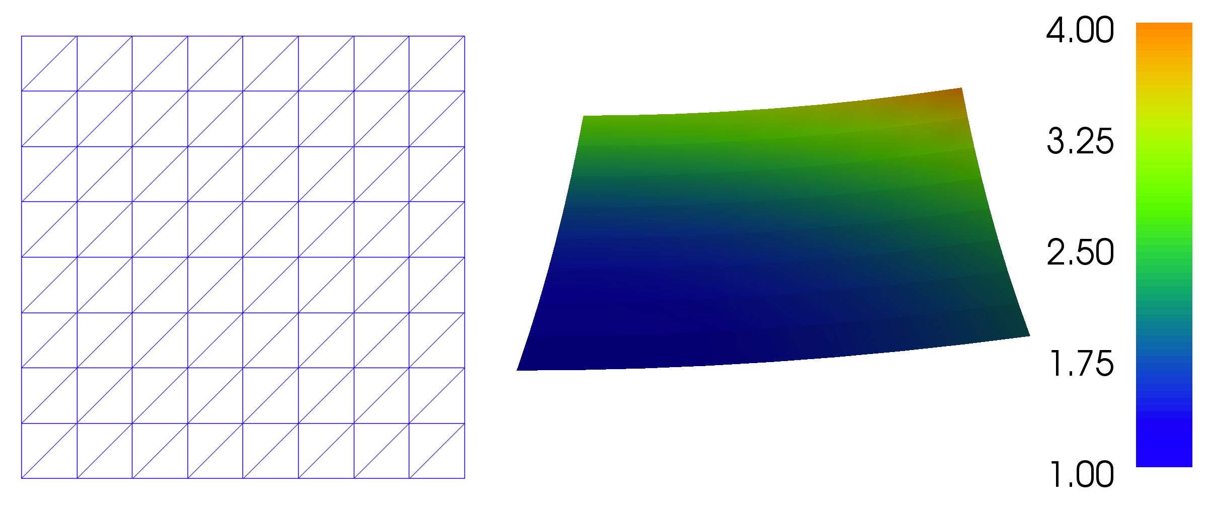
Figure 1: Plot of the mesh and the solution for the Poisson problem created using the built-in FEniCS visualization tool (plot command).

The plot command is useful for debugging and initial scientific investigations. More advanced visualizations are better created by exporting the solution to a file and using an advanced visualization tool like ParaView, as explained in the next section.

By clicking the left mouse button in the plot window, you may rotate the solution, while the right mouse button is used for zooming. Point the mouse to the Help text in the lower left corner to display a list of all available shortcut commands. The help menu may alternatively be activated by typing h in the plot window. The plot command also accepts a number of additional arguments, such as for example setting the title of the plot window:

plot(u, title='Finite element solution')
plot(mesh, title='Finite element mesh')

For detailed documentation, either run the command help(plot) in Python or pydoc fenics.plot from a terminal window.

Built-in plotting on Mac OS X and in Docker. The built-in plotting in FEniCS may not work as expected when either running on Mac OS X or when running inside a FEniCS Docker container. FEniCS supports plotting using the plot command on Mac OS X. However, the keyboard shortcuts may fail to work. When running inside a Docker container, plotting is not supported since Docker does not interact with your windowing system. For Docker users who need plotting, it is recommended to either work within a Jupyter/FEniCS notebook (command fenicsproject notebook) or rely on ParaView or other external tools for visualization.

Plotting the solution using ParaView

The simple plot command is useful for quick visualizations, but for more advanced visualizations an external tool must be used. In this section we demonstrate how to visualize solutions in ParaView. ParaView is a powerful tool for visualizing scalar and vector fields, including those computed by FEniCS.

The first step is to export the solution in VTK format:

vtkfile = File('poisson/solution.pvd')
vtkfile << u

The following steps demonstrate how to create a plot of the solution of our Poisson problem in ParaView. The resulting plot is shown in Figure 2.

Start the ParaView application.
Click File–Open... in the top menu and navigate to the directory containing the exported solution. This should be inside a subdirectory named poisson below the directory where the FEniCS Python program was started. Select the file named solution.pvd and then click OK.
Click Apply in the Properties pane on the left. This will bring up a plot of the solution.
To make a 3D plot of the solution, we will make use of one of ParaView's many filters. Click Filters–Alphabetical–Warp By Scalar in the top menu and then Apply in the Properties pane on the left. This create an elevated surface with the height determined by the solution value.
To show the original plot below the elevated surface, click the little eye icon to the left of solution.pvd in the Pipeline Browser pane on the left. Also click the little 2D button at the top of the plot window to change the visualization to 3D. This lets you interact with the plot by rotating (left mouse button) and zooming (Ctrl + left mouse button).
To show the finite element mesh, click on solution.pvd in the Pipeline Browser, navigate to Representation in the Properties pane, and select Surface With Edges. This should make the finite element mesh visible.
To change the aspect ratio of the plot, click on WarpByScalar1 in the Pipeline Browser and navigate to Scale Factor in the Properties pane. Change the value to 0.2 and click Apply. This will change the scale of the warped plot. We also unclick Orientation Axis Visibility at the bottom of the Properties pane to remove the little 3D axes in the lower left corner of the plot window. You should now see something that resembles the plot in Figure 2.
Finally, to export the visualization to a file, click File–Save Screenshot... and select a suitable file name such as poisson.png.

For more information, we refer to The ParaView Guide [27] (free PDF available), the ParaView tutorial, and the instruction video Introduction to ParaView.

Figure 2: Plot of the mesh and the solution for the Poisson problem created using ParaView.

Computing the error

Finally, we compute the error to check the accuracy of the solution. We do this by comparing the finite element solution u with the exact solution, which in this example happens to be the same as the expression u_D used to set the boundary conditions. We compute the error in two different ways. First, we compute the $ L^2 $ norm of the error, defined by $$ E = \sqrt{\int_\Omega (\ub - u)^2\dx}\tp$$ Since the exact solution is quadratic and the finite element solution is piecewise linear, this error will be nonzero. To compute this error in FEniCS, we simply write

error_L2 = errornorm(u_D, u, 'L2')

The errornorm function can also compute other error norms such as the $ H^1 $ norm. Type pydoc fenics.errornorm in a terminal window for details.

We also compute the maximum value of the error at all the vertices of the finite element mesh. As mentioned above, we expect this error to be zero to within machine precision for this particular example. To compute the error at the vertices, we first ask FEniCS to compute the value of both u_D and u at all vertices, and then subtract the results:

vertex_values_u_D = u_D.compute_vertex_values(mesh)
vertex_values_u = u.compute_vertex_values(mesh)
import numpy as np
error_max = np.max(np.abs(vertex_values_u_D - vertex_values_u))

We have here used the maximum and absolute value functions from numpy, because these are much more efficient for large arrays (a factor of 30) than Python's built-in max and abs functions.

How to check that the error vanishes. With inexact (floating point) arithmetic, the maximum error at the vertices is not zero, but should be a small number. The machine precision is about $ 10^{-16} $, but in finite element calculations, rounding errors of this size may accumulate, to produce an error larger than $ 10^{-16} $. Experiments show that increasing the number of elements and increasing the degree of the finite element polynomials increases the error. For a mesh with $ 2\times(20\times 20) $ cubic Lagrange elements (degree 3) the error is about $ 2\cdot 10^{-12} $, while for 128 linear elements the error is about $ 2\cdot 10^{-15} $.

Examining degrees of freedom and vertex values

A finite element function like $ u $ is expressed as a linear combination of basis functions $ \phi_j $, spanning the space $ V $: $$ \begin{equation} u = \sum_{j=1}^N U_j \phi_j \tag{2.13}\tp \end{equation} $$ By writing solve(a == L, u, bc) in the program, a linear system will be formed from $ a $ and $ L $, and this system is solved for the values $ U_1,\ldots,U_N $. The values $ U_1,\ldots,U_N $ are known as the degrees of freedom ("dofs") or nodal values of $ u $. For Lagrange elements (and many other element types) $ U_j $ is simply the value of $ u $ at the node with global number $ j $. The locations of the nodes and cell vertices coincide for linear Lagrange elements, while for higher-order elements there are additional nodes associated with the facets, edges and sometimes also the interior of cells.

Having u represented as a Function object, we can either evaluate u(x) at any point x in the mesh (expensive operation!), or we can grab all the degrees of freedom in the vector $ U $ directly by

nodal_values_u = u.vector()

The result is a Vector object, which is basically an encapsulation of the vector object used in the linear algebra package that is used to solve the linear system arising from the variational problem. Since we program in Python it is convenient to convert the Vector object to a standard numpy array for further processing:

array_u = nodal_values_u.array()

With numpy arrays we can write MATLAB-like code to analyze the data. Indexing is done with square brackets: array_u[j], where the index j always starts at 0. If the solution is computed with piecewise linear Lagrange elements ($ \mathsf{P}_1 $), then the size of the array array_u is equal to the number of vertices, and each array_u[j] is the value at some vertex in the mesh. However, the degrees of freedom are not necessarily numbered in the same way as the vertices of the mesh. (This is discussed in some detail in the section Examining the degrees of freedom). If we therefore want to know the values at the vertices, we need to call the function u.compute_vertex_values. This function returns the values at all the vertices of the mesh as a numpy array with the same numbering as for the vertices of the mesh, for example:

vertex_values_u = u.compute_vertex_values()

Note that for $ \mathsf{P}_1 $ elements, the arrays array_u and vertex_values_u have the same lengths and contain the same values, albeit in different order.