The Navier–Stokes equations
For the next example, we will solve the incompressible Navier–Stokes equations. This problem combines many of the challenges from our previously studied problems: time-dependence, nonlinearity, and vector-valued variables. We shall touch on a number of FEniCS topics, many of them quite advanced. But you will see that even a relatively complex algorithm such as a second-order splitting method for the incompressible Navier–Stokes equations, can be implemented with relative ease in FEniCS.
PDE problem
The incompressible Navier–Stokes equations form a system of equations for the velocity \( u \) and pressure \( p \) in an incompressible fluid: $$ \begin{align} \tag{3.29} \varrho\left(\frac{\partial u}{\partial t} + u \cdot \nabla u\right) &= \nabla\cdot\sigma(u, p) + f, \\ \tag{3.30} \nabla \cdot u &= 0. \end{align} $$ The right-hand side \( f \) is a given force per unit volume and just as for the equations of linear elasticity, \( \sigma(u, p) \) denotes the stress tensor, which for a Newtonian fluid is given by $$ \begin{equation} \sigma(u, p) = 2\mu\epsilon(u) - pI, \tag{3.31} \end{equation} $$ where \( \epsilon(u) \) is the strain-rate tensor $$ \epsilon(u) = \frac{1}{2}\left(\nabla u + (\nabla u)^T\right)\tp$$ The parameter \( \mu \) is the dynamic viscosity. Note that the momentum equation (3.29) is very similar to the elasticity equation (3.20). The difference is in the two additional terms \( \varrho(\partial u / \partial t + u \cdot \nabla u) \) and the different expression for the stress tensor. The two extra terms express the acceleration balanced by the force \( F = \nabla\cdot\sigma + f \) per unit volume in Newton's second law of motion.
Variational formulation
The Navier–Stokes equations are different from the time-dependent heat equation in that we need to solve a system of equations and this system is of a special type. If we apply the same technique as for the heat equation; that is, replacing the time derivative with a simple difference quotient, we obtain a nonlinear system of equations. This in itself is not a problem for FEniCS as we saw in the section A nonlinear Poisson equation, but the system has a so-called saddle point structure and requires special techniques (special preconditioners and iterative methods) to be solved efficiently.
Instead, we will apply a simpler and often very efficient approach, known as a splitting method. The idea is to consider the two equations (3.29) and (3.30) separately. There exist many splitting strategies for the incompressible Navier–Stokes equations. One of the oldest is the method proposed by Chorin [29] and Temam [30], often referred to as Chorin's method. We will use a modified version of Chorin's method, the so-called incremental pressure correction scheme (IPCS) due to [31] which gives improved accuracy compared to the original scheme at little extra cost.
The IPCS scheme involves three steps. First, we compute a tentative
velocity \( u^{\star} \) by advancing the momentum equation
(3.29) by a midpoint finite difference scheme in
time, but using the pressure \( p^{n} \) from the
previous time interval. We will also linearize the nonlinear convective
term by using the known velocity \( u^{n} \) from the previous time step:
\( u^{n}\cdot\nabla u^{n} \).
The variational problem for this first step is
$$
\begin{align}
\tag{3.32}
& \langle {\varrho(u^{\star} - u^{n}) / \dt},{v} \rangle
+ \langle {\varrho u^{n} \cdot \nabla u^{n}},{v} \rangle
+ \nonumber
\langle {\sigma(u^{n+\frac{1}{2}}, p^{n})},{\epsilon(v)} \rangle \\
&\quad\quad\quad\quad\quad
+ \langle {p^{n} n},{v} \rangle_{\partial\Omega}
- \langle {\mu\nabla u^{n+\frac{1}{2}}\cdot n},{v} \rangle_{\partial\Omega}
= \langle {f^{n+1}},{v} \rangle.
\tag{3.33}
\end{align}
$$
This notation, suitable for problems with many terms in the variational
formulations, requires some explanation. First, we use the short-hand
notation
$$
\inner{v}{w} = \int_{\Omega} vw \dx, \quad
\inner{v}{w}_{\partial\Omega} = \int_{\partial\Omega} vw \ds.
$$
This allows us to express the variational problem in a more compact
way. Second, we use the notation \( u^{n+\frac{1}{2}} \). This notation
refers to the value of \( u \) at the midpoint of the interval, usually
approximated by an arithmetic mean:
$$
u^{n+\frac{1}{2}} \approx (u^n + u^{n+1}) / 2.
$$
Third, we notice that the variational problem (3.32)
arises from the integration by parts of the term
\( \inner{-\nabla\cdot\sigma}{v} \). Just as for the elasticity problem in
the section The equations of linear elasticity, we obtain
$$
\inner{-\nabla\cdot\sigma}{v}
= \inner{\sigma}{\epsilon(v)}
- \inner{T}{v}_{\partial\Omega},
$$
where \( T = \sigma\cdot n \) is the boundary traction. If we solve a
problem with a free boundary, we can take \( T = 0 \) on the
boundary. However, if we compute the flow through a channel or a pipe
and want to model flow that continues into an "imaginary channel" at
the outflow, we need to treat this term with some care. The assumption
we then make is that the derivative of the velocity in the direction
of the channel is zero at the outflow, corresponding to a flow that is
"fully developed" or doesn't change significantly downstream of the
outflow. Doing so, the remaining boundary term at the outflow becomes
\( pn - \mu\nabla u \cdot n \), which is the term appearing in the
variational problem (3.32). Note that this argument and
the implementation depends on the exact definition of \( \nabla u \), as
either the matrix with components \( \partial u_i / \partial x_j \) or
\( \partial u_j / \partial x_i \). We here choose the latter, \( \partial
u_j / \partial x_i \), which means that we must use the FEniCS operator
nabla_grad for the implementation. If we use the grad operator and
the definition \( \partial u_i / \partial x_j \), we must instead keep the
terms \( pn - \mu(\nabla u)^{\top} \cdot n \)!
grad(u) vs. nabla_grad(u).
For scalar functions, \( \nabla u \) has a clear meaning as the vector
$$ \nabla u =\left(\frac{\partial u}{\partial x}, \frac{\partial u}{\partial y},
\frac{\partial u}{\partial z}\right)\tp$$
However, if \( u \) is vector-valued, the meaning is less clear.
Some sources define \( \nabla u \) as the matrix with elements
\( \partial u_j / \partial x_i \), while other sources prefer
\( \partial u_i / \partial x_j \). In FEniCS, grad(u) is defined as the
matrix with elements \( \partial u_i / \partial x_j \), which is the
natural definition of \( \nabla u \) if we think of this as the gradient or
derivative of \( u \). This way, the matrix \( \nabla u \) can be applied to
a differential \( \dx \) to give an increment \( \mathrm{d}u = \nabla u \,
\dx \). Since the alternative interpretation of \( \nabla u \) as the matrix
with elements \( \partial u_j / \partial x_i \) is very common, in
particular in continuum mechanics, FEniCS
provides the operator nabla_grad for this purpose.
For the Navier–Stokes equations, it is important to consider the
term \( u \cdot \nabla u \) which should be interpreted as the vector
\( w \) with elements
\( w_i = \sum_j \left(u_j \frac{\partial}{\partial x_j}\right) u_i
= \sum_j u_j \frac{\partial u_i}{\partial x_j} \).
This term can be implemented in FEniCS either as
grad(u)*u, since this is expression becomes
\( \sum_j \partial u_i/\partial x_j u_j \), or as
dot(u, nabla_grad(u)) since this expression becomes
\( \sum_i u_i \partial u_j/\partial x_i \). We will use the notation
dot(u, nabla_grad(u)) below since it corresponds more closely
to the standard notation \( u \cdot \nabla u \).
To be more precise, there are three different notations used for PDEs
involving gradient, divergence, and curl operators. One employs
\( \mathrm{grad}\, u \), \( \mathrm{div}\, u \), and \( \mathrm{curl}\, u \)
operators. Another employs \( \nabla u \) as a synonym for
\( \mathrm{grad}\, u \), \( \nabla\cdot u \) means \( \mathrm{div}\, u \), and
\( \nabla\times u \) is the name for \( \mathrm{curl}\, u \). The third
operates with \( \nabla u \), \( \nabla\cdot u \), and \( \nabla\times u \) in
which \( \nabla \) is a vector and, e.g., \( \nabla u \) is a dyadic
expression: \( (\nabla u)_{i,j} = \partial u_j/\partial x_i =
(\mathrm{grad}\,u)^{\top} \). The latter notation, with \( \nabla \) as a
vector operator, is often handy when deriving equations in continuum
mechanics, and if this interpretation of \( \nabla \) is the foundation of
your PDE, you must use nabla_grad, nabla_div, and nabla_curl in
FEniCS code as these operators are compatible with dyadic
computations. From the Navier–Stokes equations we can easily see
what \( \nabla \) means: if the convective term has the form \( u\cdot
\nabla u \), actually meaning \( (u\cdot\nabla) u \), then \( \nabla \) is a
vector and the implementation becomes dot(u, nabla_grad(u)) in
FEniCS, but if we see \( \nabla u\cdot u \) or \( (\mathrm{grad} u)\cdot u \),
the corresponding FEniCS expression is dot(grad(u), u).
Similarly, the divergence of a tensor field like the stress tensor
\( \sigma \) can also be expressed in two different ways, as either
div(sigma) or nabla_div(sigma). The first case corresponds to the
components \( \partial \sigma_{ij}/{\partial x_j} \) and the second to
\( \partial \sigma_{ij}/{\partial x_i} \). In general, these expressions
will be different but when the stress measure is symmetric, the
expressions have the same value.
We now move on to the second step in our splitting scheme for the incompressible Navier–Stokes equations. In the first step, we computed the tentative velocity \( u^{\star} \) based on the pressure from the previous time step. We may now use the computed tentative velocity to compute the new pressure \( p^n \): $$ \begin{equation} \tag{3.34} \langle \nabla p^{n+1}, \nabla q \rangle = \langle {\nabla p^{n}},{\nabla q} \rangle - \dt^{-1} \langle{\nabla \cdot u^{\star}},{q} \rangle. \end{equation} $$ Note here that \( q \) is a scalar-valued test function from the pressure space, whereas the test function \( v \) in (3.32) is a vector-valued test function from the velocity space.
One way to think about this step is to subtract the Navier–Stokes momentum equation (3.29) expressed in terms of the tentative velocity \( u^{\star} \) and the pressure \( p^n \) from the momentum equation expressed in terms of the velocity \( u^{n+1} \) and pressure \( p^{n+1} \). This results in the equation $$ \begin{equation} \tag{3.35} (u^{n+1} - u^{\star}) / \dt + \nabla p^{n+1} - \nabla p^n = 0. \end{equation} $$ Taking the divergence and requiring that \( \nabla \cdot u^{n+1} = 0 \) by the Navier–Stokes continuity equation (3.30), we obtain the equation \( -\nabla\cdot u^{\star} / \dt + \nabla^2 p^{n+1} - \nabla^2 p^n = 0 \), which is a Poisson problem for the pressure \( p^{n+1} \) resulting in the variational problem (3.34).
Finally, we compute the corrected velocity \( u^{n+1} \) from the equation (3.35). Multiplying this equation by a test function \( v \), we obtain $$ \begin{equation} \tag{3.36} \langle {u^{n+1}},{v} \rangle = \langle {u^{\star}},{v} \rangle - \dt \langle {\nabla(p^{n+1}-p^{n})},{v} \rangle. \end{equation} $$
In summary, we may thus solve the incompressible Navier–Stokes equations efficiently by solving a sequence of three linear variational problems in each time step.
FEniCS implementation
Test problem 1: Channel flow
As a first test problem, we compute the flow between two infinite plates, so-called channel or Poiseuille flow. As we shall see, this problem has a known analytical solution. Let \( H \) be the distance between the plates and \( L \) the length of the channel. There are no body forces.
We may scale the problem first to get rid of seemingly independent physical parameters. The physics of this problem is governed by viscous effects only, in the direction perpendicular to the flow, so a time scale should be based on diffusion accross the channel: \( t_c = H^2/\nu \). We let \( U \), some characteristic inflow velocity, be the velocity scale and \( H \) the spatial scale. The pressure scale is taken as the characteristic shear stress, \( \mu U/H \), since this is a primary example of shear flow. Inserting \( \bar x = x/H \), \( \bar y = y/H \), \( \bar z = z/H \), \( \bar u =u/U \), \( \bar p = Hp/(\mu U) \), and \( \bar t = H^2/\nu \) in the equations results in the scaled Navier–Stokes equations (dropping bars after the scaling): $$ \begin{align*} \frac{\partial u}{\partial t} + \mathrm{Re}\, u\cdot\nabla u &= -\nabla p + \nabla^2 u,\\ \nabla\cdot u &= 0\tp \end{align*} $$ Here, \( \mathrm{Re} = \varrho UH/\mu \) is the Reynolds number. Because of the time and pressure scales, which are different from convection-dominated fluid flow, the Reynolds number is associated with the convective term and not the viscosity term.
The exact solution is derived by assuming \( u=(u_x(x,y,z),0,0) \), with the \( x \) axis pointing along the channel. Since \( \nabla\cdot u=0 \), \( u \) cannot depend on \( x \). The physics of channel flow is also two-dimensional so we can omit the \( z \) coordinate (more precisely: \( \partial/\partial z=0 \)). Inserting \( u=(u_x,0,0) \) in the (scaled) governing equations gives \( u_x''(y) = \partial p/\partial x \). Differentiating this equation with respect to \( x \) shows that \( \partial^2 p/\partial^2 x =0 \) so \( \partial p/\partial x \) is a constant, here called \( -\beta \). This is the driving force of the flow and can be specified as a known parameter in the problem. Integrating \( u_x''(y)=-\beta \) over the width of the channel, \( [0,1] \), and requiring \( u=(0, 0, 0) \) at the channel walls, results in \( u_x=\frac{1}{2}\beta y(1-y) \). The characteristic inlet velocity \( U \) can be taken as the maximum inflow at \( y=1/2 \), implying \( \beta = 8 \). The length of the channel, \( L/H \) in the scaled model, has no impact on the result, so for simplicity we just compute on the unit square. Mathematically, the pressure must be prescribed at a point, but since \( p \) does not depend on \( y \), we can set \( p \) to a known value, e.g. zero, along the outlet boundary \( x=1 \). The result is \( p(x)=8(1-x) \) and \( u_x=4y(1-y) \).
The boundary conditions can be set as \( p=8 \) at \( x=0 \), \( p=0 \) at \( x=1 \) and \( u=(0, 0, 0) \) on the walls \( y=0,1 \). This defines the pressure drop and should result in unit maximum velocity at the inlet and outlet and a parabolic velocity profile without further specifications. Note that it is only meaningful to solve the Navier–Stokes equations in 2D or 3D geometries, although the underlying mathematical problem collapses to two 1D problems, one for \( u_x(y) \) and one for \( p(x) \).
The scaled model is not so easy to simulate using a standard Navier–Stokes solver with dimensions. However, one can argue that the convection term is zero, so the Re coefficient in front of this term in the scaled PDEs is not important and can be set to unity. In that case, setting \( \varrho = \mu = 1 \) in the original Navier–Stokes equations resembles the scaled model.
For a specific engineering problem one wants to simulate a specific fluid and set corresponding parameters. A general solver is therefore most naturally implemented with dimensions and the original physical parameters. However, scaling may greatly simplify numerical simulations. First of all, it shows that all fluids behave in the same way: it does not matter whether we have oil, gas, or water flowing between two plates, and it does not matter how fast the flow is (up to some criticial value of the Reynolds number where the flow becomes unstable and transitions to a complicated turbulent flow of totally different nature). This means that one simulation is enough to cover all types of channel flow! In other applications, scaling shows that it might be necessary to set just the fraction of some parameters (dimensionless numbers) rather than the parameters themselves. This simplifies exploring the input parameter space which is often the purpose of simulation. Frequently, the scaled problem is run by setting some of the input parameters with dimension to fixed values (often unity).
FEniCS implementation
Our previous examples have all started out with the creation of a mesh
and then the definition of a FunctionSpace on the mesh. For the
Navier–Stokes splitting scheme we will need to define two function
spaces, one for the velocity and one for the pressure:
V = VectorFunctionSpace(mesh, 'P', 2)
Q = FunctionSpace(mesh, 'P', 1)
The first space V is a vector-valued function space for the velocity
and the second space Q is a scalar-valued function space for the
pressure. We use piecewise quadratic elements for the velocity and
piecewise linear elements for the pressure. When creating a
VectorFunctionSpace in FEniCS, the value-dimension (the length of
the vectors) will be set equal to the geometric dimension of the
finite element mesh. One can easily create vector-valued function
spaces with other dimensions in FEniCS by adding the keyword parameter
dim:
V = VectorFunctionSpace(mesh, 'P', 2, dim=10)
Since we have two different function spaces, we need to create two sets of trial and test functions:
u = TrialFunction(V)
v = TestFunction(V)
p = TrialFunction(Q)
q = TestFunction(Q)
As we have seen in previous examples, boundaries may be defined in
FEniCS by defining Python functions that return True or False
depending on whether a point should be considered part of the
boundary, for example
def boundary(x, on_boundary):
    return near(x[0], 0)
This function defines the boundary to be all points with
\( x \)-coordinate equal to (near) zero. The near function comes from
FEniCS and performs a test with tolerance: abs(x[0] - 0) < 3E-16 so we
do not run into rounding troubles. Alternatively, we may give the
boundary definition as a string of C++ code, much like we have
previously defined expressions such as u_D = Expression('1 + x[0]*x[0]
+ 2*x[1]*x[1]', degree=2). The above definition of the boundary in
terms of a Python function may thus be replaced by a simple C++
string:
boundary = 'near(x[0], 0)'
This has the advantage of moving the computation of which nodes belong to the boundary from Python to C++, which improves the efficiency of the program.
For the current example, we will set three different boundary conditions. First, we will set \( u = 0 \) at the walls of the channel; that is, at \( y = 0 \) and \( y = 1 \). Second, we will set \( p = 8 \) at the inflow (\( x = 0 \)) and, finally, \( p = 0 \) at the outflow (\( x = 1 \)). This will result in a pressure gradient that will accelerate the flow from the initial state with zero velocity. These boundary conditions may be defined as follows:
# Define boundaries
inflow   = 'near(x[0], 0)'
outflow  = 'near(x[0], 1)'
walls    = 'near(x[1], 0) || near(x[1], 1)'

# Define boundary conditions
bcu_noslip  = DirichletBC(V, Constant((0, 0)), walls)
bcp_inflow  = DirichletBC(Q, Constant(8), inflow)
bcp_outflow = DirichletBC(Q, Constant(0), outflow)
bcu = [bcu_noslip]
bcp = [bcp_inflow, bcp_outflow]
At the end, we collect the boundary conditions for the velocity and pressure in Python lists so we can easily access them in the following computation.
We now move on to the definition of the variational forms. There are three variational problems to be defined, one for each step in the IPCS scheme. Let us look at the definition of the first variational problem. We start with some constants:
U   = 0.5*(u_n + u)
n   = FacetNormal(mesh)
f   = Constant((0, 0))
k   = Constant(dt)
mu  = Constant(mu)
rho = Constant(rho)
The next step is to set up the variational form for the first step
(3.32) in the solution process. Since the variational
problem contains a mix of known and unknown quantities we will use the
following naming convention: u is the unknown (mathematically
\( u^{n+1} \)) as a trial function in the variational form, u_ is the
most recently computed approximation (\( u^{n+1} \) available as a
Function object), u_n is \( u^n \), and the same convention goes for
p, p_ (\( p^{n+1} \)), and p_n (\( p^n \)).
# Define strain-rate tensor
def epsilon(u):
    return sym(nabla_grad(u))

# Define stress tensor
def sigma(u, p):
    return 2*mu*epsilon(u) - p*Identity(len(u))

# Define variational problem for step 1
F1 = rho*dot((u - u_n) / k, v)*dx + \
     rho*dot(dot(u_n, nabla_grad(u_n)), v)*dx \
   + inner(sigma(U, p_n), epsilon(v))*dx \
   + dot(p_n*n, v)*ds - dot(mu*nabla_grad(U)*n, v)*ds \
   - dot(f, v)*dx
a1 = lhs(F1)
L1 = rhs(F1)
Note that we take advantage of the Python programming language to
define our own operators sigma and epsilon. Using Python this way
makes it easy to extend the mathematical language of FEniCS with
special operators and constitutive laws.
Also note that FEniCS can sort out the bilinear form \( a(u,v) \) and
linear form \( L(v) \) forms by the lhs
and rhs functions. This is particularly convenient in longer and
more complicated variational forms.
The splitting scheme requires the solution of a sequence of three
variational problems in each time step. We have previously used the
built-in FEniCS function solve to solve variational problems. Under
the hood, when a user calls solve(a == L, u, bc), FEniCS will
perform the following steps:
A = assemble(A)
b = assemble(L)
bc.apply(A, b)
solve(A, u.vector(), b)
In the last step, FEniCS uses the overloaded solve function to solve
the linear system AU = b where U is the vector of degrees of
freedom for the function \( u(x) = \sum_{j=1} U_j \phi_j(x) \).
In our implementation of the splitting scheme, we will make use of these low-level commands to first assemble and then call solve. This has the advantage that we may control when we assemble and when we solve the linear system. In particular, since the matrices for the three variational problems are all time-independent, it makes sense to assemble them once and for all outside of the time-stepping loop:
A1 = assemble(a1)
A2 = assemble(a2)
A3 = assemble(a3)
Within the time-stepping loop, we may then assemble only the right-hand side vectors, apply boundary conditions, and call the solve function as here for the first of the three steps:
# Time-stepping
t = 0
for n in range(num_steps):

    # Update current time
    t += dt

    # Step 1: Tentative velocity step
    b1 = assemble(L1)
    [bc.apply(b1) for bc in bcu]
    solve(A1, u_.vector(), b1)
Notice the Python list comprehension [bc.apply(b1) for bc in bcu]
which iterates over all bc in the list bcu. This is a convenient
and compact way to construct a loop that applies
all boundary conditions in a single line. Also, the code works if
we add more Dirichlet boundary conditions in the future. Note that
the boundary conditions only need to be applied to the right-hand side
vectors as they have already been applied to the matrices (not shown).
Finally, let us look at an important detail in how we use parameters
such as the time step dt in the definition of our variational
problems. Since we might want to change these later, for example if we
want to experiment with smaller or larger time steps, we wrap these
using a FEniCS Constant:
k = Constant(dt)
The assembly of matrices and vectors in FEniCS is based on code
generation. This means that whenever we change a variational problem,
FEniCS will have to generate new code, which may take a little
time. New code will also be generated and compiled when a float value
for the time step is changed. By wrapping this parameter using
Constant, FEniCS will treat the parameter as a generic constant and
not as a specific numerical value, which prevents repeated code
generation. In the case of the time step, we choose a new name k
instead of dt for the Constant since we also want to use the
variable dt as a Python float as part of the time-stepping.
The complete code for simulating 2D channel flow with FEniCS can be found in the file ft07_navier_stokes_channel.py.
Verification
We compute the error at the nodes as we have done before to verify
that our implementation is correct. Our Navier–Stokes solver computes
the solution to the time-dependent incompressible Navier–Stokes
equations, starting from the initial condition \( u = (0, 0) \). We have
not specified the initial condition explicitly in our solver which
means that FEniCS will initialize all variables, in particular the
previous and current velocities u_n and u_, to zero. Since the
exact solution is quadratic, we expect the solution to be exact to
within machine precision at the nodes at infinite time. For our
implementation, the error quickly approaches zero and is approximately
\( 10^{-6} \) at time \( T = 10 \).
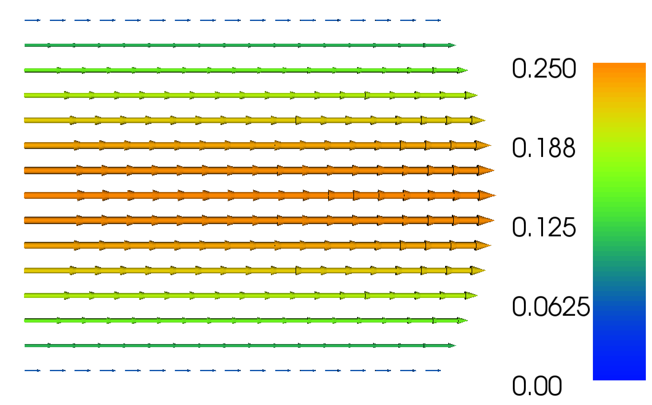
Figure 7: Plot of the velocity profile at the final time for the Navier–Stokes channel flow example.
Test problem 2: Flow past a cylinder
We now turn our attention to a more challenging problem: flow past a circular cylinder. The geometry and parameters are taken from problem DFG 2D-2 in the FEATFLOW/1995-DFG benchmark suite and is illustrated in Figure 8. The kinematic viscosity is given by \( \nu = 0.001 = \mu/\varrho \) and the inflow velocity profile is specified as $$ u(x, y, t) = \left(1.5 \cdot \frac{4y(0.41 - y)}{0.41^2}, 0\right), $$ which has a maximum magnitude of \( 1.5 \) at \( y = 0.41/2 \). We do not use any scaling for this problem since all exact parameters are known.
Figure 8: Geometry for the flow past a cylinder test problem. Notice the slightly perturbed and unsymmetric geometry.

FEniCS implementation
So far all our domains have been simple shapes such as a unit square or
a rectangular box. A number of such simple meshes may be created
using the built-in mesh classes in FEniCS
(UnitIntervalMesh,
UnitSquareMesh,
UnitCubeMesh,
IntervalMesh,
RectangleMesh,
BoxMesh).
FEniCS supports the creation of more complex meshes via a technique
called constructive solid geometry (CSG), which lets us define
geometries in terms of simple shapes (primitives) and set operations:
union, intersection, and set difference. The set operations are
encoded in FEniCS using the operators + (union), * (intersection),
and - (set difference). To access the CSG functionality in FEniCS,
one must import the FEniCS module mshr which provides the
extended meshing functionality of FEniCS.
The geometry for the cylinder flow test problem can be defined easily by first defining the rectangular channel and then subtracting the circle:
channel = Rectangle(Point(0, 0), Point(2.2, 0.41))
cylinder = Circle(Point(0.2, 0.2), 0.05)
domain = channel - cylinder
We may then create the mesh by calling the function generate_mesh:
mesh = generate_mesh(domain, 64)
Here the argument 64 indicates that we want to resolve the geometry
with 64 cells across its diameter (the channel length).
To solve the cylinder test problem, we only need to make a few minor changes to the code we wrote for the channel flow test case. Besides defining the new mesh, the only change we need to make is to modify the boundary conditions and the time step size. The boundaries are specified as follows:
inflow   = 'near(x[0], 0)'
outflow  = 'near(x[0], 2.2)'
walls    = 'near(x[1], 0) || near(x[1], 0.41)'
cylinder = 'on_boundary && x[0]>0.1 && x[0]<0.3 && x[1]>0.1 && x[1]<0.3'
The last line may seem cryptic before you catch the idea: we want to pick
out all boundary points (on_boundary) that also lie within the 2D
domain \( [0.1,0.3]\times [0.1,0.3] \), see Figure 8. The only possible points are then the points on the
circular boundary!
In addition to these essential changes, we will make a number of small changes to improve our solver. First, since we need to choose a relatively small time step to compute the solution (a time step that is too large will make the solution blow up) we add a progress bar so that we can follow the progress of our computation. This can be done as follows:
progress = Progress('Time-stepping')
set_log_level(PROGRESS)

# Time-stepping
t = 0.0
for n in range(num_steps):

    # Update current time
    t += dt

    # Place computation here

    # Update progress bar
    progress.update(t / T)
set_log_level(PROGRESS) which is essential to
make FEniCS actually display the progress bar. FEniCS is actually
quite informative about what is going on during a computation but the
amount of information printed to screen depends on the current log
level. Only messages with a priority higher than or equal to the
current log level will be displayed. The predefined log levels in
FEniCS are
DBG,
TRACE,
PROGRESS,
INFO,
WARNING,
ERROR, and
CRITICAL. By default, the log level is set to INFO which means
that messages at level DBG, TRACE, and PROGRESS will not be
printed. Users may print messages using the FEniCS functions info,
warning, and error which will print messages at the obvious log
level (and in the case of error also throw an exception and
exit). One may also use the call log(level, message) to print a
message at a specific log level.
Since the system(s) of linear equations are significantly larger than
for the simple channel flow test problem, we choose to use an
iterative method instead of the default direct (sparse) solver used by
FEniCS when calling solve. Efficient solution of linear systems
arising from the discretization of PDEs requires the choice of both a
good iterative (Krylov subspace) method and a good
preconditioner. For this problem, we will simply use the biconjugate
gradient stabilized method (BiCGSTAB) and the conjugate gradient method. This can be done by adding the
keywords bicgstab or cg in the call to solve. We also specify
suitable preconditioners to speed up the computations:
solve(A1, u1.vector(), b1, 'bicgstab', 'hypre_amg')
solve(A2, p1.vector(), b2, 'bicgstab', 'hypre_amg')
solve(A3, u1.vector(), b3, 'cg', 'sor')
Finally, to be able to postprocess the computed solution in ParaView,
we store the solution to a file in each time step. We have previously
created files with the suffix .pvd for this purpose. In the example
program
ft04_heat_gaussian.py,
we first created a file named heat_gaussian/solution.pvd and then
saved the solution in each time step using
vtkfile << (u, t)
For the present example, we will instead choose to save the solution
to XDMF format. This file format works similarly to the .pvd files
we have seen earlier but has several advantages. First, the storage is
much more efficient, both in terms of speed and file sizes. Second,
.xdmf files work in parallell, both for writing and reading
(postprocessing). Much like .pvd files, the actual data will not be
stored in the .xdmf file itself, but will instead be stored in a
(single) separate data file with the suffix .hdf5 which is an
advanced file format designed for high-performance computing.
We create the XDMF files as follows:
xdmffile_u = XDMFFile('navier_stokes_cylinder/velocity.xdmf')
xdmffile_p = XDMFFile('navier_stokes_cylinder/pressure.xdmf')
In each time step, we may then store the velocity and pressure by
xdmffile_u.write(u, t)
xdmffile_p.write(p, t)
We also store the solution using a FEniCS TimeSeries. This allows us
to store the solution not for visualization, but for later reuse in a
computation as we will see in the next section. Using a TimeSeries
it is easy and efficient to read in solutions from certain points in
time during a simulation. The TimeSeries class also uses the HDF5
file format for efficient storage and access to data.
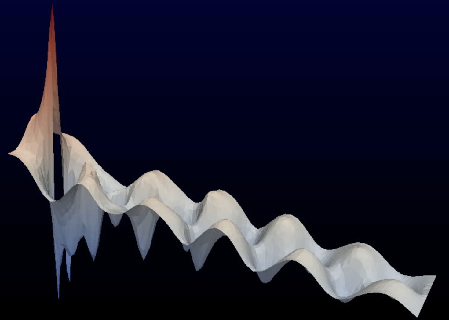
Figures 9 and 10 show the velocity and pressure at final time visualized in ParaView. For the visualization of the velocity, we have used the Glyph filter to visualize the vector velocity field. For the visualization of the pressure, we have used the Warp By Scalar filter.
Figure 9: Plot of the velocity for the cylinder test problem at final time.
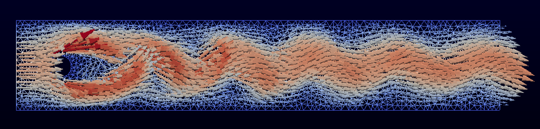
Figure 10: Plot of the pressure for the cylinder test problem at final time.
The complete code for the cylinder test problem looks as follows:
from fenics import *
from mshr import *
import numpy as np

T = 5.0            # final time
num_steps = 5000   # number of time steps
dt = T / num_steps # time step size
mu = 0.001         # dynamic viscosity
rho = 1            # density

# Create mesh
channel = Rectangle(Point(0, 0), Point(2.2, 0.41))
cylinder = Circle(Point(0.2, 0.2), 0.05)
domain = channel - cylinder
mesh = generate_mesh(domain, 64)

# Define function spaces
V = VectorFunctionSpace(mesh, 'P', 2)
Q = FunctionSpace(mesh, 'P', 1)

# Define boundaries
inflow   = 'near(x[0], 0)'
outflow  = 'near(x[0], 2.2)'
walls    = 'near(x[1], 0) || near(x[1], 0.41)'
cylinder = 'on_boundary && x[0]>0.1 && x[0]<0.3 && x[1]>0.1 && x[1]<0.3'

# Define inflow profile
inflow_profile = ('4.0*1.5*x[1]*(0.41 - x[1]) / pow(0.41, 2)', '0')

# Define boundary conditions
bcu_inflow = DirichletBC(V, Expression(inflow_profile, degree=2), inflow)
bcu_walls = DirichletBC(V, Constant((0, 0)), walls)
bcu_cylinder = DirichletBC(V, Constant((0, 0)), cylinder)
bcp_outflow = DirichletBC(Q, Constant(0), outflow)
bcu = [bcu_inflow, bcu_walls, bcu_cylinder]
bcp = [bcp_outflow]

# Define trial and test functions
u = TrialFunction(V)
v = TestFunction(V)
p = TrialFunction(Q)
q = TestFunction(Q)

# Define functions for solutions at previous and current time steps
u_n = Function(V)
u_  = Function(V)
p_n = Function(Q)
p_  = Function(Q)

# Define expressions used in variational forms
U  = 0.5*(u_n + u)
n  = FacetNormal(mesh)
f  = Constant((0, 0))
k  = Constant(dt)
mu = Constant(mu)
rho = Constant(rho)

# Define symmetric gradient
def epsilon(u):
    return sym(nabla_grad(u))

# Define stress tensor
def sigma(u, p):
    return 2*mu*epsilon(u) - p*Identity(len(u))

# Define variational problem for step 1
F1 = rho*dot((u - u_n) / k, v)*dx \
   + rho*dot(dot(u_n, nabla_grad(u_n)), v)*dx \
   + inner(sigma(U, p_n), epsilon(v))*dx \
   + dot(p_n*n, v)*ds - dot(mu*nabla_grad(U)*n, v)*ds \
   - dot(f, v)*dx
a1 = lhs(F1)
L1 = rhs(F1)

# Define variational problem for step 2
a2 = dot(nabla_grad(p), nabla_grad(q))*dx
L2 = dot(nabla_grad(p_n), nabla_grad(q))*dx - (1/k)*div(u_)*q*dx

# Define variational problem for step 3
a3 = dot(u, v)*dx
L3 = dot(u_, v)*dx - k*dot(nabla_grad(p_ - p_n), v)*dx

# Assemble matrices
A1 = assemble(a1)
A2 = assemble(a2)
A3 = assemble(a3)

# Apply boundary conditions to matrices
[bc.apply(A1) for bc in bcu]
[bc.apply(A2) for bc in bcp]

# Create XDMF files for visualization output
xdmffile_u = XDMFFile('navier_stokes_cylinder/velocity.xdmf')
xdmffile_p = XDMFFile('navier_stokes_cylinder/pressure.xdmf')

# Create time series (for use in reaction_system.py)
timeseries_u = TimeSeries('navier_stokes_cylinder/velocity_series')
timeseries_p = TimeSeries('navier_stokes_cylinder/pressure_series')

# Save mesh to file (for use in reaction_system.py)
File('navier_stokes_cylinder/cylinder.xml.gz') << mesh

# Create progress bar
progress = Progress('Time-stepping')
set_log_level(PROGRESS)

# Time-stepping
t = 0
for n in range(num_steps):

    # Update current time
    t += dt

    # Step 1: Tentative velocity step
    b1 = assemble(L1)
    [bc.apply(b1) for bc in bcu]
    solve(A1, u_.vector(), b1, 'bicgstab', 'hypre_amg')

    # Step 2: Pressure correction step
    b2 = assemble(L2)
    [bc.apply(b2) for bc in bcp]
    solve(A2, p_.vector(), b2, 'bicgstab', 'hypre_amg')

    # Step 3: Velocity correction step
    b3 = assemble(L3)
    solve(A3, u_.vector(), b3, 'cg', 'sor')

    # Plot solution
    plot(u_, title='Velocity')
    plot(p_, title='Pressure')

    # Save solution to file (XDMF/HDF5)
    xdmffile_u.write(u_, t)
    xdmffile_p.write(p_, t)

    # Save nodal values to file
    timeseries_u.store(u_.vector(), t)
    timeseries_p.store(p_.vector(), t)

    # Update previous solution
    u_n.assign(u_)
    p_n.assign(p_)

    # Update progress bar
    progress.update(t / T)
    print('u max:', u_.vector().array().max())

# Hold plot
interactive()
This program can be found in the file ft08_navier_stokes_cylinder.py. The reader should be advised that this example program is considerably more demanding than our previous examples in terms of CPU time and memory, but it should be possible to run the program on a reasonably modern laptop.