Generating meshes with subdomains
So far, we have worked mostly with simple meshes (the unit square) and
defined boundaries and subdomains in terms of simple geometric tests
like \( x = 0 \) or \( y \leq 0.5 \). For more complex geometries, it is not
realistic to specify boundaries and subdomains in this way. Instead,
the boundaries and subdomains must be defined as part of the mesh
generation process. We will now look at how to use the FEniCS mesh
generation tool mshr to generate meshes and define subdomains.
PDE problem
We will again solve the Poisson equation, but this time for a different application. Consider an iron cylinder with copper wires wound around the cylinder as in Figure 13. Through the copper wires a static current \( J = 1\,\mathrm{A} \) is flowing and we want to compute the magnetic field \( B \) in the iron cylinder, the copper wires, and the surrounding vacuum.
Figure 13: Cross-section of an iron cylinder with copper wires wound around the cylinder, here with \( n = 8 \) windings. The inner circles are cross-sections of the copper wire coming up ("north") and the outer circles are cross-sections of the copper wire going down into the plane ("south").

First, we simplify the problem to a 2D problem. We can do this by assuming that the cylinder extends far along the \( z \)-axis and as a consequence the field is virtually independent of the \( z \)-coordinate. Next, we consider Maxwell's equation to derive a Poisson equation for the magnetic field (or rather its potential): $$ \begin{align} \nabla\cdot D &= \varrho, \tag{4.13}\\ \nabla\cdot B &= 0, \tag{4.14}\\ \nabla\times E &= -\frac{\partial B}{\partial t}, \tag{4.15}\\ \nabla\times H &= \frac{\partial D}{\partial t} + J. \tag{4.16} \end{align} $$ Here, \( D \) is the displacement field, \( B \) is the magnetic field, \( E \) is the electric field, and \( H \) is the magnetizing field. In addition to Maxwell's equations, we also need a constitutive relation between \( B \) and \( H \), $$ \begin{equation} B = \mu H, \tag{4.17} \end{equation} $$ which holds for an isotropic linear magnetic medium. Here, \( \mu \) is the magnetic permeability of the material. Now, since \( B \) is solenoidal (divergence free) according to Maxwell's equations, we know that \( B \) must be the curl of some vector field \( A \). This field is called the magnetic vector potential. Since the problem is static and thus \( \partial D/\partial t = 0 \), it follows that $$ \begin{equation} J = \nabla \times H = \nabla \times (\mu^{-1} B) = \nabla \times (\mu^{-1} \nabla \times A) = -\nabla \cdot (\mu^{-1} \nabla A). \tag{4.18} \end{equation} $$ In the last step, we have expanded the second derivatives and used the gauge freedom of \( A \) to simplify the equations to a simple vector-valued Poisson problem for the magnetic vector potential; if \( B = \nabla \times A \), then \( B = \nabla \times (A + \nabla \psi) \) for any scalar field \( \psi \) (the gauge function). For the current problem, we thus need to solve the following 2D Poisson problem for the \( z \)-component \( A_z \) of the magnetic vector potential: $$ \begin{align} - \nabla \cdot (\mu^{-1} \nabla A_z) &= J_z \quad \text{in } \Real^2, \tag{4.19}\\ \lim_{|(x, y)| \rightarrow \infty} A_z &= 0. \tag{4.20} \end{align} $$ Since we cannot solve this problem on an infinite domain, we will truncate the domain using a large disk and set \( A_z = 0 \) on the boundary. The current \( J_z \) is set to \( +1\,\mathrm{A} \) in the interior set of circles (copper wire cross-sections) and to \( -1\,\mathrm{A} \) in the exterior set of circles in Figure 13.
Once the magnetic vector potential has been computed, we can compute the magnetic field \( B = B(x, y) \) by $$ \begin{align} B(x, y) = \left(\frac{\partial A_z}{\partial y}, -\frac{\partial A_z}{\partial x}\right). \tag{4.21} \end{align} $$
Variational formulation
The variational problem is derived as before by multiplying the PDE with a test function \( v \) and integrating by parts. Since the boundary integral vanishes due to the Dirichlet condition, we obtain $$ \begin{equation} \int_{\Omega} \mu^{-1} \nabla A_z \cdot \nabla v \dx = \int_{\Omega} J_z v \dx, \tag{4.22} \end{equation} $$ or, in other words, \( a(A_z, v) = L(v) \) with $$ \begin{align} a(A_z, v) &= \int_{\Omega} \mu^{-1} \nabla A_z \cdot \nabla v \dx, \tag{4.23}\\ L(v) &= \int_{\Omega} J_z v \dx. \tag{4.24} \end{align} $$
FEniCS implementation
The first step is to generate a mesh for the geometry described in
Figure 13. We let \( a \) and \( b \) be the
inner and outer radii of the iron cylinder and let \( c_1 \) and \( c_2 \)
be the radii of the two concentric distributions of copper wire
cross-sections. Furthermore, we let \( r \) be the radius of a copper
wire, \( R \) be the radius of our domain, and \( n \) be the number of
windings (giving a total of \( 2n \) copper-wire cross-sections). This
geometry can be described easily using mshr and a little bit of
Python programming:
# Define geometry for background
domain = Circle(Point(0, 0), R)

# Define geometry for iron cylinder
cylinder = Circle(Point(0, 0), b) - Circle(Point(0, 0), a)

# Define geometry for wires (N = North (up), S = South (down))
angles_N = [i*2*pi/n for i in range(n)]
angles_S = [(i + 0.5)*2*pi/n for i in range(n)]
wires_N = [Circle(Point(c_1*cos(v), c_1*sin(v)), r) for v in angles_N]
wires_S = [Circle(Point(c_2*cos(v), c_2*sin(v)), r) for v in angles_S]
The mesh that we generate will be a mesh of the entire disk with
radius \( R \) but we need the mesh generation to respect the internal
boundaries defined by the iron cylinder and the copper wires. We also
want mshr to label the subdomains so that we can easily specify
material parameters (\( \mu \)) and currents. To do this, we use the
mshr function set_subdomain as follows:
# Set subdomain for iron cylinder
domain.set_subdomain(1, cylinder)

# Set subdomains for wires
for (i, wire) in enumerate(wires_N):
    domain.set_subdomain(2 + i, wire)
for (i, wire) in enumerate(wires_S):
    domain.set_subdomain(2 + n + i, wire)
Once the subdomains have been created, we can generate the mesh:
mesh = generate_mesh(domain, 32)
A detail of the mesh is shown in Figure 14.
Figure 14: Plot of (part of) the mesh generated for the magnetostatics test problem. The subdomains for the iron cylinder and copper wires are clearly visible.

The mesh generated with mshr will contain information about the
subdomains we have defined. To use this information in the definition of
our variational problem and subdomain-dependent parameters, we will need to
create a MeshFunction that marks the subdomains. This can be easily
created by a call to the member function mesh.domains, which holds
the subdomain data generated by mshr:
markers = MeshFunction('size_t', mesh, 2, mesh.domains())
This line creates a MeshFunction with unsigned integer values (the
subdomain numbers) with dimension 2, which is the cell dimension for
this 2D problem.
We can now use the markers as we have done before to redefine the
integration measure dx:
dx = Measure('dx', domain=mesh, subdomain_data=markers)
Integrals over subdomains can then be expressed by dx(0), dx(1),
and so on. We use this to define the current \( J_z = \pm 1\,\mathrm{A} \)
in the copper wires:
J_N = Constant(1.0)
J_S = Constant(-1.0)
A_z = TrialFunction(V)
v = TestFunction(V)
a = (1 / mu)*dot(grad(A_z), grad(v))*dx
L_N = sum(J_N*v*dx(i) for i in range(2, 2 + n))
L_S = sum(J_S*v*dx(i) for i in range(2 + n, 2 + 2*n))
L = L_N + L_S
The permeability is defined as an Expression that depends on the
subdomain number:
class Permeability(Expression):
    def __init__(self, markers, **kwargs):
        self.markers = markers
    def eval_cell(self, values, x, cell):
        if self.markers[cell.index] == 0:
            values[0] = 4*pi*1e-7 # vacuum
        elif self.markers[cell.index] == 1:
            values[0] = 1e-5      # iron (should really be 6.3e-3)
        else:
            values[0] = 1.26e-6   # copper

mu = Permeability(markers, degree=1)
As seen in this code snippet, we have used a somewhat less extreme value for the magnetic permeability of iron. This is to make the solution a little more interesting. It would otherwise be completely dominated by the field in the iron cylinder.
Finally, when \( A_z \) has been computed, we can compute the magnetic field:
W = VectorFunctionSpace(mesh, 'P', 1)
B = project(as_vector((A_z.dx(1), -A_z.dx(0))), W)
We use as_vector to interpret
(A_z.dx(1), -A_z.dx(0)) as a vector in the sense of the UFL
form language, and not as a Python tuple. The resulting plots of the
magnetic vector potential and magnetic field are shown in Figures
15 and
16.
Figure 15: Plot of the \( z \)-component \( A_z \) of the magnetic vector potential.
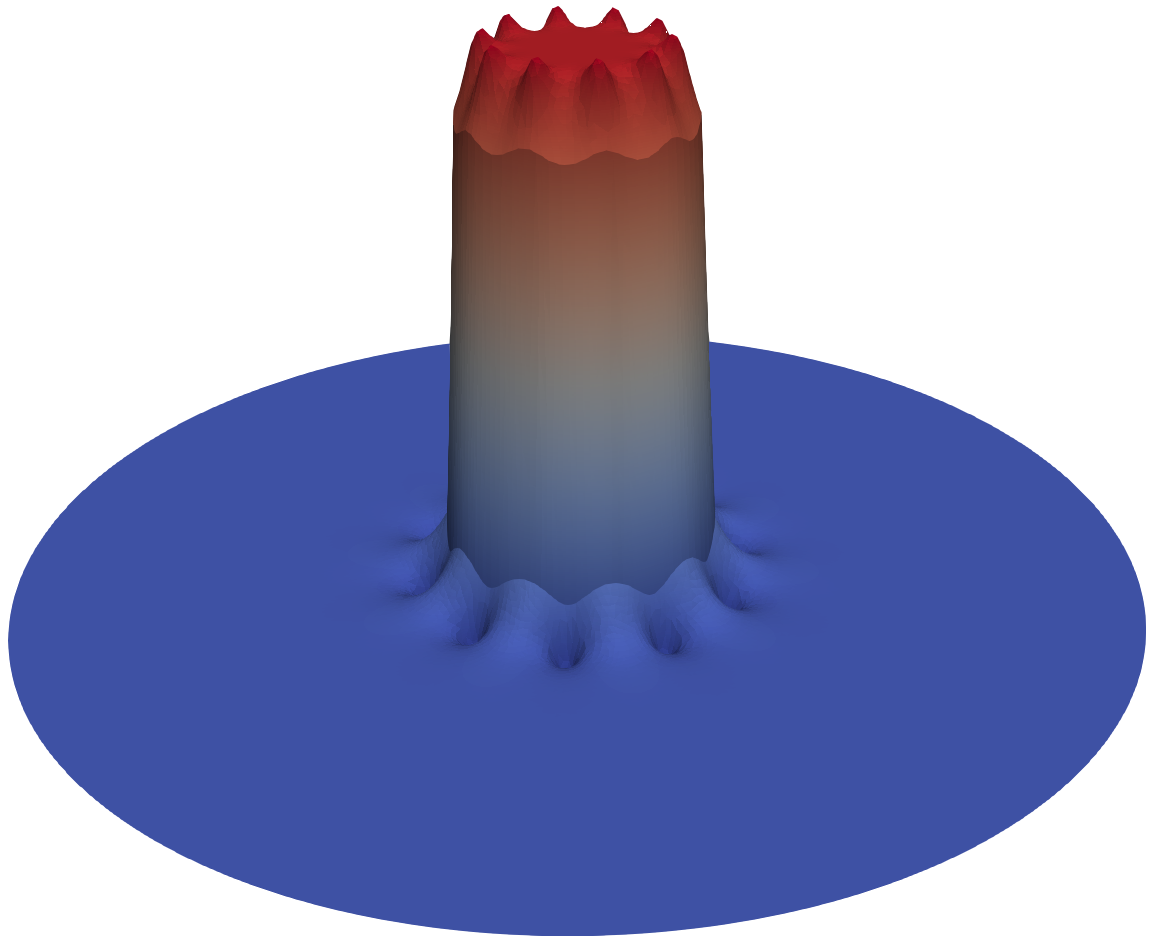
Figure 16: Plot of the magnetic field \( B \) in the \( xy \)-plane.

The complete code for computing the magnetic field follows below.
from fenics import *
from mshr import *
from math import sin, cos, pi

a = 1.0   # inner radius of iron cylinder
b = 1.2   # outer radius of iron cylinder
c_1 = 0.8 # radius for inner circle of copper wires
c_2 = 1.4 # radius for outer circle of copper wires
r = 0.1   # radius of copper wires
R = 5.0   # radius of domain
n = 10    # number of windings

# Define geometry for background
domain = Circle(Point(0, 0), R)

# Define geometry for iron cylinder
cylinder = Circle(Point(0, 0), b) - Circle(Point(0, 0), a)

# Define geometry for wires (N = North (up), S = South (down))
angles_N = [i*2*pi/n for i in range(n)]
angles_S = [(i + 0.5)*2*pi/n for i in range(n)]
wires_N = [Circle(Point(c_1*cos(v), c_1*sin(v)), r) for v in angles_N]
wires_S = [Circle(Point(c_2*cos(v), c_2*sin(v)), r) for v in angles_S]

# Set subdomain for iron cylinder
domain.set_subdomain(1, cylinder)

# Set subdomains for wires
for (i, wire) in enumerate(wires_N):
    domain.set_subdomain(2 + i, wire)
for (i, wire) in enumerate(wires_S):
    domain.set_subdomain(2 + n + i, wire)

# Create mesh
mesh = generate_mesh(domain, 128)

# Define function space
V = FunctionSpace(mesh, 'P', 1)

# Define boundary condition
bc = DirichletBC(V, Constant(0), 'on_boundary')

# Define subdomain markers and integration measure
markers = MeshFunction('size_t', mesh, 2, mesh.domains())
dx = Measure('dx', domain=mesh, subdomain_data=markers)

# Define current densities
J_N = Constant(1.0)
J_S = Constant(-1.0)

# Define magnetic permeability
class Permeability(Expression):
    def __init__(self, markers, **kwargs):
        self.markers = markers
    def eval_cell(self, values, x, cell):
        if self.markers[cell.index] == 0:
            values[0] = 4*pi*1e-7 # vacuum
        elif self.markers[cell.index] == 1:
            values[0] = 1e-5      # iron (should really be 6.3e-3)
        else:
            values[0] = 1.26e-6   # copper

mu = Permeability(markers, degree=1)

# Define variational problem
A_z = TrialFunction(V)
v = TestFunction(V)
a = (1 / mu)*dot(grad(A_z), grad(v))*dx
L_N = sum(J_N*v*dx(i) for i in range(2, 2 + n))
L_S = sum(J_S*v*dx(i) for i in range(2 + n, 2 + 2*n))
L = L_N + L_S

# Solve variational problem
A_z = Function(V)
solve(a == L, A_z, bc)

# Compute magnetic field (B = curl A)
W = VectorFunctionSpace(mesh, 'P', 1)
B = project(as_vector((A_z.dx(1), -A_z.dx(0))), W)

# Plot solution
plot(A_z)
plot(B)

# Save solution to file
vtkfile_A_z = File('magnetostatics/potential.pvd')
vtkfile_B = File('magnetostatics/field.pvd')
vtkfile_A_z << A_z
vtkfile_B << B

# Hold plot
interactive()
This example program can be found in the file ft11_magnetostatics.py.