7. Poisson equation
This demo illustrates how to:
- Solve a linear partial differential equation
- Create and apply Dirichlet boundary conditions
- Define Expressions
- Define a FunctionSpace
- Create a SubDomain
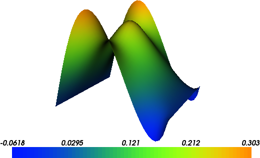
The solution for \(u\) in this demo will look as follows:
7.1. Equation and problem definition
The Poisson equation is the canonical elliptic partial differential equation. For a domain \(\Omega \subset \mathbb{R}^n\) with boundary \(\partial \Omega = \Gamma_{D} \cup \Gamma_{N}\), the Poisson equation with particular boundary conditions reads:
Here, \(f\) and \(g\) are input data and \(n\) denotes the outward directed boundary normal. The most standard variational form of Poisson equation reads: find \(u \in V\) such that
where \(V\) is a suitable function space and
The expression \(a(u, v)\) is the bilinear form and \(L(v)\) is the linear form. It is assumed that all functions in \(V\) satisfy the Dirichlet boundary conditions (\(u = 0 \ {\rm on} \ \Gamma_{D}\)).
In this demo, we shall consider the following definitions of the input functions, the domain, and the boundaries:
- \(\Omega = [0,1] \times [0,1]\) (a unit square)
- \(\Gamma_{D} = \{(0, y) \cup (1, y) \subset \partial \Omega\}\) (Dirichlet boundary)
- \(\Gamma_{N} = \{(x, 0) \cup (x, 1) \subset \partial \Omega\}\) (Neumann boundary)
- \(g = \sin(5x)\) (normal derivative)
- \(f = 10\exp(-((x - 0.5)^2 + (y - 0.5)^2) / 0.02)\) (source term)
7.2. Implementation
The implementation is split in two files: a form file containing the definition of the variational forms expressed in UFL and a C++ file containing the actual solver.
Running this demo requires the files: main.cpp,
Poisson.ufl and CMakeLists.txt.
7.2.1. UFL form file
The first step is to define the variational problem at hand. We define
the variational problem in UFL terms in a separate form file
Poisson.ufl. We begin by defining the finite element:
element = FiniteElement("Lagrange", triangle, 1)
The first argument to FiniteElement is the finite element
family, the second argument specifies the domain, while the third
argument specifies the polynomial degree. Thus, in this case, our
element element consists of first-order, continuous Lagrange basis
functions on triangles (or in order words, continuous piecewise linear
polynomials on triangles).
Next, we use this element to initialize the trial and test functions (\(u\) and \(v\)) and the coefficient functions (\(f\) and \(g\)):
u = TrialFunction(element)
v = TestFunction(element)
f = Coefficient(element)
g = Coefficient(element)
Finally, we define the bilinear and linear forms according to the variational formulation of the equations:
a = inner(grad(u), grad(v))*dx
L = f*v*dx + g*v*ds
Before the form file can be used in the C++ program, it must be compiled using FFC by running (on the command-line):
ffc -l dolfin Poisson.ufl
Note the flag -l dolfin which tells FFC to generate
DOLFIN-specific wrappers that make it easy to access the generated
code from within DOLFIN.
7.2.2. C++ program
The main solver is implemented in the main.cpp file.
At the top we include the DOLFIN header file and the generated header file “Poisson.h” containing the variational forms for the Poisson equation. For convenience we also include the DOLFIN namespace.
#include <dolfin.h>
#include "Poisson.h"

using namespace dolfin;
Then follows the definition of the coefficient functions (for
\(f\) and \(g\)), which are derived from the
Expression class in DOLFIN.
// Source term (right-hand side)
class Source : public Expression
{
  void eval(Array<double>& values, const Array<double>& x) const
  {
    double dx = x[0] - 0.5;
    double dy = x[1] - 0.5;
    values[0] = 10*exp(-(dx*dx + dy*dy) / 0.02);
  }
};

// Normal derivative (Neumann boundary condition)
class dUdN : public Expression
{
  void eval(Array<double>& values, const Array<double>& x) const
  {
    values[0] = sin(5*x[0]);
  }
};
The DirichletBoundary is derived from the SubDomain
class and defines the part of the boundary to which the Dirichlet
boundary condition should be applied.
// Sub domain for Dirichlet boundary condition
class DirichletBoundary : public SubDomain
{
  bool inside(const Array<double>& x, bool on_boundary) const
  {
    return x[0] < DOLFIN_EPS or x[0] > 1.0 - DOLFIN_EPS;
  }
};
Inside the main function, we begin by defining a mesh of the
domain. As the unit square is a very standard domain, we can use a
built-in mesh provided by the class UnitSquareMesh. In order
to create a mesh consisting of 32 x 32 squares with each square
divided into two triangles, and the finite element space (specified in
the form file) defined relative to this mesh, we do as follows
// Create mesh and function space
UnitSquareMesh mesh(32, 32);
Poisson::FunctionSpace V(mesh);
Now, the Dirichlet boundary condition (\(u = 0\)) can be created
using the class DirichletBC. A DirichletBC
takes three arguments: the function space the boundary condition
applies to, the value of the boundary condition, and the part of the
boundary on which the condition applies. In our example, the function
space is V, the value of the boundary condition (0.0) can
represented using a Constant, and the Dirichlet boundary
is defined by the class DirichletBoundary listed
above. The definition of the Dirichlet boundary condition then looks
as follows:
// Define boundary condition
Constant u0(0.0);
DirichletBoundary boundary;
DirichletBC bc(V, u0, boundary);
Next, we define the variational formulation by initializing the
bilinear and linear forms (\(a\), \(L\)) using the previously
defined FunctionSpace V. Then we can create the
source and boundary flux term (\(f\), \(g\)) and attach these
to the linear form.
// Define variational forms
Poisson::BilinearForm a(V, V);
Poisson::LinearForm L(V);
Source f;
dUdN g;
L.f = f;
L.g = g;
Now, we have specified the variational forms and can consider the
solution of the variational problem. First, we need to define a
Function u to store the solution. (Upon
initialization, it is simply set to the zero function.) Next, we can
call the solve function with the arguments a == L, u and
bc as follows:
// Compute solution
Function u(V);
solve(a == L, u, bc);
The function u will be modified during the call to solve. A
Function can be manipulated in various ways, in
particular, it can be plotted and saved to file. Here, we output the
solution to a VTK file (using the suffix .pvd) for later
visualization and also plot it using the plot command:
// Save solution in VTK format
File file("poisson.pvd");
file << u;

// Plot solution
plot(u);
7.3. Complete code
7.3.1. Complete UFL file
element = FiniteElement("Lagrange", triangle, 1)

u = TrialFunction(element)
v = TestFunction(element)
f = Coefficient(element)
g = Coefficient(element)

a = inner(grad(u), grad(v))*dx
L = f*v*dx + g*v*ds
7.3.2. Complete main file
#include <dolfin.h>
#include "Poisson.h"

using namespace dolfin;

// Source term (right-hand side)
class Source : public Expression
{
  void eval(Array<double>& values, const Array<double>& x) const
  {
    double dx = x[0] - 0.5;
    double dy = x[1] - 0.5;
    values[0] = 10*exp(-(dx*dx + dy*dy) / 0.02);
  }
};

// Normal derivative (Neumann boundary condition)
class dUdN : public Expression
{
  void eval(Array<double>& values, const Array<double>& x) const
  {
    values[0] = sin(5*x[0]);
  }
};

// Sub domain for Dirichlet boundary condition
class DirichletBoundary : public SubDomain
{
  bool inside(const Array<double>& x, bool on_boundary) const
  {
    return x[0] < DOLFIN_EPS or x[0] > 1.0 - DOLFIN_EPS;
  }
};

int main()
{
  // Create mesh and function space
  UnitSquareMesh mesh(32, 32);
  Poisson::FunctionSpace V(mesh);

  // Define boundary condition
  Constant u0(0.0);
  DirichletBoundary boundary;
  DirichletBC bc(V, u0, boundary);

  // Define variational forms
  Poisson::BilinearForm a(V, V);
  Poisson::LinearForm L(V);

  Source f;
  dUdN g;
  L.f = f;
  L.g = g;

  // Compute solution
  Function u(V);
  solve(a == L, u, bc);

  // Save solution in VTK format
  File file("poisson.pvd");
  file << u;

  // Plot solution
  plot(u);
  interactive();

  return 0;
}