6. Incompressible Navier-Stokes equations
This demo solves the incompressible Navier-Stokes equations. It illustrates how to:
- Implement a splitting method where different fields are coupled via a set of partial differential equations
- Use different iterative solvers and different preconditioners for different steps of the solution process
- Use time-dependent Expressions
- Set boundary conditions based on geometric constraints
- Perform time-stepping
6.1. Equation and solution method
We consider the incompressible Navier-Stokes equations on a domain \(\Omega \subset \mathbb{R}^2\), consisting of a pair of momentum and continuity equations:
Here, \(u\) is the unknown velocity, \(p\) is the unknown pressure, \(\nu\) is the kinematic viscosity, and \(f\) is a given source. There exist many solution strategies for the incompressible Navier-Stokes equations. One of the oldest is the splitting method proposed by Chorin (1968) and Temam (1969), often refered to as Chorin’s method.
In Chorin’s method, one first ignores the pressure in the momentum equation and computes the tentative velocity \(u_h^{\star}\) according to:
Here, \(\langle \cdot, \cdot \rangle\) denotes the \(L^2(\Omega)\) inner product. Subsequently, the velocity is projected to the space of divergence free fields. This step may be obtained by subtracting the variational problem for the tentative velocity \(u_h^{\star}\) from the incompressible Navier-Stokes equations and using the continuity equation. One obtains the following pair of equations for computing the velocity \(u_h^n\) and pressure \(p_h^n\) at time \(t = t_n\) based on the tentative velocity \(u_h^{\star}\):
6.2. Problem definition
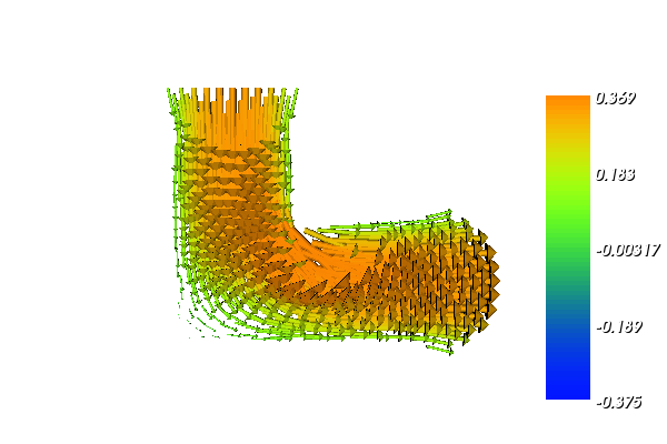
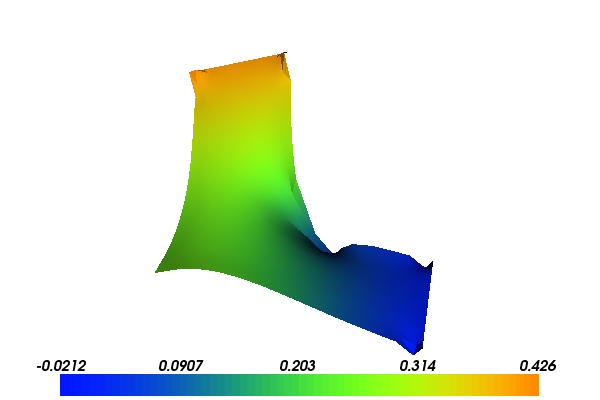
In this demo, we solve the incompressible Navier-Stokes equations on an L-shaped domain. The L-shape is the subset of the unit square obtained by removing the upper right quadrant.
The flow is driven by an oscillating pressure \(p_{\mathrm{in}}(t) = \sin 3t\) at the inflow \(y = 1\) while the pressure is kept constant \(p_{\mathrm{out}} = 0\) at the outflow \(x = 1\).
At the inflow and outflow, we impose free flow (“do nothing”) boundary conditions for the velocity and no-slip boundary conditions on the remaining boundary.
The (kinematic) viscosity is set to \(\nu = 0.01\), the time step is \(\Delta t = 0.01\) and the length of the time interval is \(T = 3\). The solution is computed using continuous vector-valued piecewise quadratics for the velocity, and continuous scalar piecewise linears for the pressure (the Taylor-Hood elements).
With the above input the solution for the velocity \(u\) and pressure \(p\) will look as follows:
6.3. Implementation
The implementation is split in four files: three form files containing the definition of the variational forms expressed in UFL and a C++ file containing the actual solver.
Running this demo requires the files: main.cpp,
TentativeVelocity.ufl, VelocityUpdate.ufl,
PressureUpdate.ufl and CMakeLists.txt.
6.3.1. UFL form files
The variational forms for the three steps of Chorin’s method are implemented in three separate UFL form files.
The variational problem for the tentative velocity is implemented as follows:
# Define function spaces (P2-P1)
V = VectorElement("Lagrange", triangle, 2)
Q = FiniteElement("Lagrange", triangle, 1)

# Define trial and test functions
u = TrialFunction(V)
v = TestFunction(V)

# Define coefficients
k  = Constant(triangle)
u0 = Coefficient(V)
f  = Coefficient(V)
nu = 0.01

# Define bilinear and linear forms
eq = (1/k)*inner(u - u0, v)*dx + inner(grad(u0)*u0, v)*dx + \
    nu*inner(grad(u), grad(v))*dx - inner(f, v)*dx
a = lhs(eq)
L = rhs(eq)
The variational problem for the pressure update is implemented as follows:
# Define function spaces (P2-P1)
V = VectorElement("Lagrange", triangle, 2)
Q = FiniteElement("Lagrange", triangle, 1)

# Define trial and test functions
p = TrialFunction(Q)
q = TestFunction(Q)

# Define coefficients
k  = Constant(triangle)
u1 = Coefficient(V)

# Define bilinear and linear forms
a = inner(grad(p), grad(q))*dx
L = -(1/k)*div(u1)*q*dx
The variational problem for the velocity update is implemented as follows:
# Define function spaces (P2-P1)
V = VectorElement("Lagrange", triangle, 2)
Q = FiniteElement("Lagrange", triangle, 1)

# Define trial and test functions
u = TrialFunction(V)
v = TestFunction(V)

# Define coefficients
k  = Constant(triangle)
u1 = Coefficient(V)
p1 = Coefficient(Q)

# Define bilinear and linear forms
a = inner(u, v)*dx
L = inner(u1, v)*dx - k*inner(grad(p1), v)*dx
Before the form files can be used in the C++ program, they must be compiled using FFC:
ffc -l dolfin TentativeVelocity.ufl
ffc -l dolfin VelocityUpdate.ufl
ffc -l dolfin PressureUpdate.ufl
Note the flag -l dolfin which tells FFC to generate
DOLFIN-specific wrappers that make it easy to access the generated
code from within DOLFIN.
6.3.2. C++ program
In the C++ program, main.cpp, we start by including
dolfin.h and the generated header files:
#include <dolfin.h>
#include "TentativeVelocity.h"
#include "PressureUpdate.h"
#include "VelocityUpdate.h"
To be able to use classes and functions from the DOLFIN namespace directly, we write
using namespace dolfin;
Next, we define the subdomains that we will use to specify boundary
conditions. We do this by defining subclasses of
SubDomain and overloading the function inside:
// Define noslip domain
class NoslipDomain : public SubDomain
{
  bool inside(const Array<double>& x, bool on_boundary) const
  {
    return (on_boundary &&
            (x[0] < DOLFIN_EPS || x[1] < DOLFIN_EPS ||
             (x[0] > 0.5 - DOLFIN_EPS && x[1] > 0.5 - DOLFIN_EPS)));
  }
};

// Define inflow domain
class InflowDomain : public SubDomain
{
  bool inside(const Array<double>& x, bool on_boundary) const
  { return x[1] > 1.0 - DOLFIN_EPS; }
};

// Define inflow domain
class OutflowDomain : public SubDomain
{
  bool inside(const Array<double>& x, bool on_boundary) const
  { return x[0] > 1.0 - DOLFIN_EPS; }
};
We also define a subclass of Expression which we will use
to specify the time-dependent boundary value for the pressure at the
inflow.
// Define pressure boundary value at inflow
class InflowPressure : public Expression
{
public:

  // Constructor
  InflowPressure() : t(0) {}

  // Evaluate pressure at inflow
  void eval(Array<double>& values, const Array<double>& x) const
  { values[0] = sin(3.0*t); }

  // Current time
  double t;

};
Note that the member variable t is not automatically updated
during time-stepping, so we must remember to manually update the value
of the current time in each time step.
Once we have defined all classes we will use to write our program, we start our C++ program by writing
int main()
{
For the parallel case, we turn off log messages from processes other than the the root process to avoid excessive output:
// Print log messages only from the root process in parallel
parameters["std_out_all_processes"] = false;
We then load the mesh for the L-shaped domain from file:
// Load mesh from file
Mesh mesh("../lshape.xml.gz");
We next define a pair of function spaces \(V\) and \(Q\) for the velocity and pressure, and test and trial functions on these spaces:
// Create function spaces
VelocityUpdate::FunctionSpace V(mesh);
PressureUpdate::FunctionSpace Q(mesh);
The time step and the length of the interval are defined by:
// Set parameter values
double dt = 0.01;
double T = 3;
We next define the time-dependent pressure boundary value, and zero scalar and vector constants that will be used for boundary conditions below.
// Define values for boundary conditions
InflowPressure p_in;
Constant zero(0);
Constant zero_vector(0, 0);
Before we can define our boundary conditions, we also need to instantiate the classes we defined above for the boundary subdomains:
// Define boundary conditions
DirichletBC noslip(V, zero_vector, noslip_domain);
DirichletBC inflow(Q, p_in, inflow_domain);
DirichletBC outflow(Q, zero, outflow_domain);
std::vector<DirichletBC*> bcu;
bcu.push_back(&noslip);
std::vector<DirichletBC*> bcp;
bcp.push_back(&inflow);
bcp.push_back(&outflow);
We may now define the boundary conditions for the velocity and pressure. We define one no-slip boundary condition for the velocity and a pair of boundary conditions for the pressure at the inflow and outflow boundaries:
// Define boundary conditions
DirichletBC noslip(V, zero_vector, noslip_domain);
DirichletBC inflow(Q, p_in, inflow_domain);
DirichletBC outflow(Q, zero, outflow_domain);
std::vector<DirichletBC*> bcu;
bcu.push_back(&noslip);
std::vector<DirichletBC*> bcp;
bcp.push_back(&inflow);
bcp.push_back(&outflow);
We collect the boundary conditions in the two arrays bcu and
bcp so that we may easily iterate over them below when we apply
the boundary conditions. This makes it easy to add new boundary
conditions or use this demo program to solve the Navier-Stokes
equations on other geometries.
We next define the functions and the coefficients that will be used below:
// Create functions
Function u0(V);
Function u1(V);
Function p1(Q);

// Create coefficients
Constant k(dt);
Constant f(0, 0);
The next step is now to define the variational problems for the three steps of Chorin’s method. We do this by instantiating the classes generated from our UFL form files:
// Create forms
TentativeVelocity::BilinearForm a1(V, V);
TentativeVelocity::LinearForm L1(V);
PressureUpdate::BilinearForm a2(Q, Q);
PressureUpdate::LinearForm L2(Q);
VelocityUpdate::BilinearForm a3(V, V);
VelocityUpdate::LinearForm L3(V);
Since the forms depend on coefficients, we have to attach the coefficients defined above to the appropriate forms:
// Set coefficients
a1.k = k; L1.k = k; L1.u0 = u0; L1.f = f;
L2.k = k; L2.u1 = u1;
L3.k = k; L3.u1 = u1; L3.p1 = p1;
Since the bilinear forms do not depend on any coefficients that change during time-stepping, the corresponding matrices remain constant. We may therefore assemble these before the time-stepping begins:
// Assemble matrices
Matrix A1, A2, A3;
assemble(A1, a1);
assemble(A2, a2);
assemble(A3, a3);

// Create vectors
Vector b1, b2, b3;

// Use amg preconditioner if available
const std::string prec(has_krylov_solver_preconditioner("amg") ? "amg" : "default");
We also created the vectors that will be used below to assemble right-hand sides.
During time-stepping, we will store the solution in VTK format
(readable by MayaVi and Paraview). We therefore create a pair of files
that can be used to store the solution. Specifying the .pvd suffix
signals that the solution should be stored in VTK format:
// Create files for storing solution
File ufile("results/velocity.pvd");
File pfile("results/pressure.pvd");
The time-stepping loop is now implemented as follows:
// Time-stepping
double t = dt;
while (t < T + DOLFIN_EPS)
{
  // Update pressure boundary condition
  p_in.t = t;
We remember to update the current time for the time-dependent pressure boundary value.
For each of the three steps of Chorin’s method, we assemble the right-hand side, apply boundary conditions, and solve a linear system. Note the different use of preconditioners. Incomplete LU factorization is used for the computation of the tentative velocity and the velocity update, while algebraic multigrid is used for the pressure equation if available:
// Compute tentative velocity step
begin("Computing tentative velocity");
assemble(b1, L1);
for (std::size_t i = 0; i < bcu.size(); i++)
  bcu[i]->apply(A1, b1);
solve(A1, *u1.vector(), b1, "gmres", "default");
end();

// Pressure correction
begin("Computing pressure correction");
assemble(b2, L2);
for (std::size_t i = 0; i < bcp.size(); i++)
  bcp[i]->apply(A2, b2);
solve(A2, *p1.vector(), b2, "cg", prec);
end();

// Velocity correction
begin("Computing velocity correction");
assemble(b3, L3);
for (std::size_t i = 0; i < bcu.size(); i++)
  bcu[i]->apply(A3, b3);
solve(A3, *u1.vector(), b3, "gmres", "default");
end();
Note the use of begin and end; these improve the readability
of the output from the program by adding indentation to diagnostic
messages.
At the end of the time-stepping loop, we store the solution to file and update values for the next time step:
// Save to file
ufile << u1;
pfile << p1;

// Move to next time step
u0 = u1;
t += dt;
Finally, we plot the solution and the program is finished:
  // Plot solution
  plot(p1, "Pressure");
  plot(u1, "Velocity");
  interactive();

  return 0;
}
6.4. Complete code
6.4.1. Complete UFL files
# Define function spaces (P2-P1)
V = VectorElement("Lagrange", triangle, 2)
Q = FiniteElement("Lagrange", triangle, 1)

# Define trial and test functions
u = TrialFunction(V)
v = TestFunction(V)

# Define coefficients
k  = Constant(triangle)
u0 = Coefficient(V)
f  = Coefficient(V)
nu = 0.01

# Define bilinear and linear forms
eq = (1/k)*inner(u - u0, v)*dx + inner(grad(u0)*u0, v)*dx + \
    nu*inner(grad(u), grad(v))*dx - inner(f, v)*dx
a  = lhs(eq)
L  = rhs(eq)
# Define function spaces (P2-P1)
V = VectorElement("Lagrange", triangle, 2)
Q = FiniteElement("Lagrange", triangle, 1)

# Define trial and test functions
u = TrialFunction(V)
v = TestFunction(V)

# Define coefficients
k  = Constant(triangle)
u1 = Coefficient(V)
p1 = Coefficient(Q)

# Define bilinear and linear forms
a = inner(u, v)*dx
L = inner(u1, v)*dx - k*inner(grad(p1), v)*dx
# Define function spaces (P2-P1)
V = VectorElement("Lagrange", triangle, 2)
Q = FiniteElement("Lagrange", triangle, 1)

# Define trial and test functions
p = TrialFunction(Q)
q = TestFunction(Q)

# Define coefficients
k  = Constant(triangle)
u1 = Coefficient(V)

# Define bilinear and linear forms
a = inner(grad(p), grad(q))*dx
L = -(1/k)*div(u1)*q*dx
6.4.2. Complete main file
#include <dolfin.h>
#include "TentativeVelocity.h"
#include "PressureUpdate.h"
#include "VelocityUpdate.h"

using namespace dolfin;

// Define noslip domain
class NoslipDomain : public SubDomain
{
  bool inside(const Array<double>& x, bool on_boundary) const
  {
    return (on_boundary &&
            (x[0] < DOLFIN_EPS || x[1] < DOLFIN_EPS ||
             (x[0] > 0.5 - DOLFIN_EPS && x[1] > 0.5 - DOLFIN_EPS)));
  }
};

// Define inflow domain
class InflowDomain : public SubDomain
{
  bool inside(const Array<double>& x, bool on_boundary) const
  { return x[1] > 1.0 - DOLFIN_EPS; }
};

// Define inflow domain
class OutflowDomain : public SubDomain
{
  bool inside(const Array<double>& x, bool on_boundary) const
  { return x[0] > 1.0 - DOLFIN_EPS; }
};

// Define pressure boundary value at inflow
class InflowPressure : public Expression
{
public:

  // Constructor
  InflowPressure() : t(0) {}

  // Evaluate pressure at inflow
  void eval(Array<double>& values, const Array<double>& x) const
  { values[0] = sin(3.0*t); }

  // Current time
  double t;

};

int main()
{
  // Print log messages only from the root process in parallel
  parameters["std_out_all_processes"] = false;

  // Load mesh from file
  Mesh mesh("../lshape.xml.gz");

  // Create function spaces
  VelocityUpdate::FunctionSpace V(mesh);
  PressureUpdate::FunctionSpace Q(mesh);

  // Set parameter values
  double dt = 0.01;
  double T = 3;

  // Define values for boundary conditions
  InflowPressure p_in;
  Constant zero(0);
  Constant zero_vector(0, 0);

  // Define subdomains for boundary conditions
  NoslipDomain noslip_domain;
  InflowDomain inflow_domain;
  OutflowDomain outflow_domain;

  // Define boundary conditions
  DirichletBC noslip(V, zero_vector, noslip_domain);
  DirichletBC inflow(Q, p_in, inflow_domain);
  DirichletBC outflow(Q, zero, outflow_domain);
  std::vector<DirichletBC*> bcu;
  bcu.push_back(&noslip);
  std::vector<DirichletBC*> bcp;
  bcp.push_back(&inflow);
  bcp.push_back(&outflow);

  // Create functions
  Function u0(V);
  Function u1(V);
  Function p1(Q);

  // Create coefficients
  Constant k(dt);
  Constant f(0, 0);

  // Create forms
  TentativeVelocity::BilinearForm a1(V, V);
  TentativeVelocity::LinearForm L1(V);
  PressureUpdate::BilinearForm a2(Q, Q);
  PressureUpdate::LinearForm L2(Q);
  VelocityUpdate::BilinearForm a3(V, V);
  VelocityUpdate::LinearForm L3(V);

  // Set coefficients
  a1.k = k; L1.k = k; L1.u0 = u0; L1.f = f;
  L2.k = k; L2.u1 = u1;
  L3.k = k; L3.u1 = u1; L3.p1 = p1;

  // Assemble matrices
  Matrix A1, A2, A3;
  assemble(A1, a1);
  assemble(A2, a2);
  assemble(A3, a3);

  // Create vectors
  Vector b1, b2, b3;

  // Use amg preconditioner if available
  const std::string prec(has_krylov_solver_preconditioner("amg") ? "amg" : "default");

  // Create files for storing solution
  File ufile("results/velocity.pvd");
  File pfile("results/pressure.pvd");

  // Time-stepping
  double t = dt;
  while (t < T + DOLFIN_EPS)
  {
    // Update pressure boundary condition
    p_in.t = t;

    // Compute tentative velocity step
    begin("Computing tentative velocity");
    assemble(b1, L1);
    for (std::size_t i = 0; i < bcu.size(); i++)
      bcu[i]->apply(A1, b1);
    solve(A1, *u1.vector(), b1, "gmres", "default");
    end();

    // Pressure correction
    begin("Computing pressure correction");
    assemble(b2, L2);
    for (std::size_t i = 0; i < bcp.size(); i++)
      bcp[i]->apply(A2, b2);
    solve(A2, *p1.vector(), b2, "cg", prec);
    end();

    // Velocity correction
    begin("Computing velocity correction");
    assemble(b3, L3);
    for (std::size_t i = 0; i < bcu.size(); i++)
      bcu[i]->apply(A3, b3);
    solve(A3, *u1.vector(), b3, "gmres", "default");
    end();

    // Save to file
    ufile << u1;
    pfile << p1;

    // Move to next time step
    u0 = u1;
    t += dt;
    cout << "t = " << t << endl;
  }

  // Plot solution
  plot(p1, "Pressure");
  plot(u1, "Velocity");
  interactive();

  return 0;
}