2. Cahn-Hilliard equation
This example demonstrates the solution of a particular nonlinear time-dependent fourth-order equation, known as the Cahn-Hilliard equation. In particular it demonstrates the use of
- The built-in Newton solver
- Advanced use of the base class
NonlinearProblem - Automatic linearisation
- A mixed finite element method
- The \(\theta\)-method for time-dependent equations
- User-defined Expressions as Python classes
- Form compiler options
- Interpolation of functions
2.1. Equation and problem definition
The Cahn-Hilliard equation is a parabolic equation and is typically used to model phase separation in binary mixtures. It involves first-order time derivatives, and second- and fourth-order spatial derivatives. The equation reads:
where \(c\) is the unknown field, the function \(f\) is usually non-convex in \(c\) (a fourth-order polynomial is commonly used), \(n\) is the outward directed boundary normal, and \(M\) is a scalar parameter.
2.1.1. Mixed form
The Cahn-Hilliard equation is a fourth-order equation, so casting it in a weak form would result in the presence of second-order spatial derivatives, and the problem could not be solved using a standard Lagrange finite element basis. A solution is to rephrase the problem as two coupled second-order equations:
The unknown fields are now \(c\) and \(\mu\). The weak (variational) form of the problem reads: find \((c, \mu) \in V \times V\) such that
2.1.2. Time discretisation
Before being able to solve this problem, the time derivative must be dealt with. Apply the \(\theta\)-method to the mixed weak form of the equation:
where \(dt = t_{n+1} - t_{n}\) and \(\mu_{n+\theta} = (1-\theta) \mu_{n} + \theta \mu_{n+1}\). The task is: given \(c_{n}\) and \(\mu_{n}\), solve the above equation to find \(c_{n+1}\) and \(\mu_{n+1}\).
2.1.3. Demo parameters
The following domains, functions and time stepping parameters are used in this demo:
- \(\Omega = (0, 1) \times (0, 1)\) (unit square)
- \(f = 100 c^{2} (1-c)^{2}\)
- \(\lambda = 1 \times 10^{-2}\)
- \(M = 1\)
- \(dt = 5 \times 10^{-6}\)
- \(\theta = 0.5\)
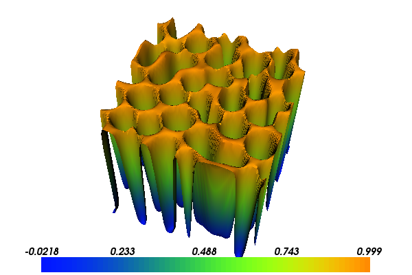
With the above input the solution for \(c\) will look as follows:
2.2. Implementation
The implementation is split in three files: two form files containing the definition of the variational forms expressed in UFL and a C++ file containing the actual solver.
Running this demo requires the files: main.cpp,
CahnHilliard2D.ufl, CahnHilliard3D.ufl and
CMakeLists.txt.
2.2.1. UFL form files
The UFL code for this problem in two and three dimensions are in
CahnHilliard2D.ufl and CahnHilliard3D.ufl respectively.
However, only the two dimensional case is explained in detail in the following.
First, a mixed function spaces of linear Lagrange functions on triangles is created:
P1 = FiniteElement("Lagrange", triangle, 1)
ME = P1*P1
On the mixed space, trial and test functions are defined:
du   = TrialFunction(ME)
q, v = TestFunctions(ME)
The test functions have been split into components.
Coefficient functions are now defined for the current solution (the most recent guess) and the solution from the beginning of the time step. Further, these functions (and the trial function) are split into their components:
u   = Coefficient(ME)  # current solution
u0  = Coefficient(ME)  # solution from previous converged step

# Split mixed functions
dc, dmu = split(du)
c,  mu  = split(u)
c0, mu0 = split(u0)
Various model parameters can be specified using the class
Constant. This means that their value can be changed
without recompiling the UFL file. Lastly, the value of
\(\mu_{n+\theta}\) is computed.
lmbda    = Constant(triangle) # surface energy parameter
dt       = Constant(triangle) # time step
theta    = Constant(triangle) # time stepping parameter

# mu_(n+theta)
mu_mid = (1-theta)*mu0 + theta*mu
The chemical potential \(df/dc\) will be computed using automated differentiation:
# Compute the chemical potential df/dc
c    = variable(c)
f    = 100*c**2*(1-c)**2
dfdc = diff(f, c)
Here, the first line declares that c is a variable that some
function can be differentiated with respect to. The next line is the
function \(f\) defined in the problem statement, and the third
line performs the differentiation of f with respect to the
variable c.
The linear forms for the two equations can be summed into one form
L. We wish to drive the residual of this form to zero during the
solution process. The directional derivative of L can be computed
automatically, by calling derivative, to form the bilinear form
a representing the Jacobian matrix:
F0 = c*q*dx  - c0*q*dx   + dt*dot(grad(mu_mid), grad(q))*dx
F1 = mu*v*dx - dfdc*v*dx - lmbda*dot(grad(c), grad(v))*dx
F = F0 + F1

J = derivative(F, u, du)
2.2.2. C++ program
The first lines of this solver include the DOLFIN header files
and the two files generated by the form compiler, and the DOLFIN
namespace is used:
#include <dolfin.h>
#include "CahnHilliard2D.h"
#include "CahnHilliard3D.h"

using namespace dolfin;
The class InitialConditions defines the initial conditions for the
solver. In the constructor, the random number generator is seeded
using the rank (process number) so that different processes will
generate different sequences when running in parallel. The eval
function evaluates the initial condition. The first value ([0])
corresponds to \(c\) and the second value ([1]) corresponds to
\(\mu\):
// Initial conditions
class InitialConditions : public Expression
{
public:

  InitialConditions() : Expression(2)
  {
     dolfin::seed(2 + dolfin::MPI::rank(MPI_COMM_WORLD));
  }

  void eval(Array<double>& values, const Array<double>& x) const
  {
    values[0]= 0.63 + 0.02*(0.5 - dolfin::rand());
    values[1]= 0.0;
  }
};
The next class is a subclass of NonlinearProblem. A
NonlinearProblem object can be passed to a
NewtonSolver to be solved. The requirements of a
NonlinearProblem subclass are that it provides the
function void F(GenericVector& b, const GenericVector& x) for
computing the residual vector and the function void J(GenericMatrix&
A, const GenericVector& x) for computing the Jacobian matrix. The
below class is designed to work for two different generated forms (2D
and 3D), with the appropriate form chosen based on the geometric
dimension of the mesh. The makes the class more complicated than would
be the case if it supported a single form type. The class is first
declared as a subclass of cpp:class:NonlinearProblem:
// User defined nonlinear problem
class CahnHilliardEquation : public NonlinearProblem
{
public:
Its constructor takes the various arguments which are required
to create the forms, and it calls a the templated private member
function init:
// Constructor
CahnHilliardEquation(const Mesh& mesh, const Constant& dt,
const Constant& theta, const Constant& lambda)
{
// Initialize class (depending on geometric dimension of the mesh).
// Unfortunately C++ does not allow namespaces as template arguments
if (mesh.geometry().dim() == 2)
{
init<CahnHilliard2D::FunctionSpace, CahnHilliard2D::JacobianForm,
CahnHilliard2D::ResidualForm>(mesh, dt, theta, lambda);
}
else if (mesh.geometry().dim() == 3)
{
init<CahnHilliard3D::FunctionSpace, CahnHilliard3D::JacobianForm,
CahnHilliard3D::ResidualForm>(mesh, dt, theta, lambda);
}
else
error("Cahn-Hilliard model is programmed for 2D and 3D only.");
}
The function F computes the residual vector, which corresponds to
assembly of the form L:
// User defined residual vector
void F(GenericVector& b, const GenericVector& x)
{
// Assemble RHS (Neumann boundary conditions)
Assembler assembler;
assembler.assemble(b, *L);
}
The function J computes the Jacobian matrix, which corresponds to
the assembly of the form a.
// User defined assemble of Jacobian
void J(GenericMatrix&
A, const GenericVector& x)
{
// Assemble system
Assembler assembler;
assembler.assemble(A, *a);
}
The following two functions are helper functions which allow access to the solution vectors:
// Return solution function
Function& u()
{ return *_u; }
// Return solution function
Function& u0()
{ return *_u0; }
The private init function is responsible for creating the forms
and functions associated with the problem. It is a templated function
so that the 2D and 3D cases can be handled with the same code.
Firstly, a shared pointer to a FunctionSpace (X) is
created. Then two shared pointers _u and _u0 are set to point
to Function s from the space V. A shared pointer is
used so that the function space is not destroyed when the constructor
exits. (The function space will not be destroyed until there are no
more Functions or Forms that point to it.) Using the function space
V, bilinear and linear forms are created using new, and the
coefficient functions are attached. These forms are then wrapped in a
shared pointer (using the reset function) which will take care of
eventually destroying the forms. Finally, _u is set equal to the
initial condition (by interpolation).
private:
template<class X, class Y, class Z>
void init(const Mesh& mesh, const Constant& dt, const Constant& theta,
const Constant& lambda)
{
// Create function space and functions
std::shared_ptr<X> V(new X(mesh));
_u.reset(new Function(V));
_u0.reset(new Function(V));
// Create forms and attach functions
Y* _a = new Y(V, V);
Z* _L = new Z(V);
_a->u = *_u; _a->lmbda = lambda; _a->dt = dt; _a->theta = theta;
_L->u = *_u; _L->u0 = *_u0;
_L->lmbda = lambda; _L->dt = dt; _L->theta = theta;
// Wrap pointers in a smart pointer
a.reset(_a);
L.reset(_L);
// Set solution to intitial condition
InitialConditions u_initial;
*_u = u_initial;
}
The CahnHilliardEquation class stores the data required for
computing the residual vector and the Jacobian matrix as private data:
// Function space, forms and functions
boost::scoped_ptr<Form> a;
boost::scoped_ptr<Form> L;
boost::scoped_ptr<Function> _u;
boost::scoped_ptr<Function> _u0;
};
The main program is started, and declared such that it can accept
command line arguments. Such are parsed to init:
int main(int argc, char* argv[])
{
init(argc, argv);
A mesh is then created with 97 (96 + 1) vertices in each direction:
// Mesh
UnitSquareMesh mesh(96, 96);
A set of constants (required for the assembling of the forms) and two scalars (to be used in the time stepping) are then declared:
// Time stepping and model parameters
Constant dt(5.0e-6);
Constant theta(0.5);
Constant lambda(1.0e-2);
double t = 0.0;
double T = 50*dt;
A CahnHilliardEquation object is created, which will be used in conjunction
with a Newton solver, and references to solution functions are
declared:
// Create user-defined nonlinear problem
CahnHilliardEquation cahn_hilliard(mesh, dt, theta, lambda);
// Solution functions
Function& u = cahn_hilliard.u();
Function& u0 = cahn_hilliard.u0();
A Newton solver is created which will use a LU linear solver, and various solver parameters are set:
// Create nonlinear solver and set parameters
NewtonSolver newton_solver;
newton_solver.parameters["linear_solver"] = "lu";
newton_solver.parameters["convergence_criterion"] = "incremental";
newton_solver.parameters["maximum_iterations"] = 10;
newton_solver.parameters["relative_tolerance"] = 1e-6;
newton_solver.parameters["absolute_tolerance"] = 1e-15;
A file is created for saving the solution at each time step in VTK format. The data will be compressed to reduce the file size.
// Save initial condition to file
File file("cahn_hilliard.pvd", "compressed");
file << u[0];
The solution process is based on stepping forward in time. At the
beginning of each time step, time is incremented and \(u_{n}
\leftarrow u_{n+1}\). The Newton solver is then used to solve the
nonlinear equation and the first component of the solution (u[0])
is saved to a file, along with the time t.
// Solve
while (t < T)
{
// Update for next time step
t += dt;
*u0.vector() = *u.vector();
// Solve
newton_solver.solve(cahn_hilliard, *u.vector());
// Save function to file
file << std::pair<const Function*, double>(&(u[0]), t);
}
The final result is plotted to the screen and the program is finished.
// Plot solution
plot(u[0]);
interactive();
return 0;
}
2.3. Complete code
2.3.1. Complete UFL files
P1 = FiniteElement("Lagrange", triangle, 1)
ME = P1*P1
du = TrialFunction(ME)
q, v = TestFunctions(ME)
u = Coefficient(ME) # current solution
u0 = Coefficient(ME) # solution from previous converged step
# Split mixed functions
dc, dmu = split(du)
c, mu = split(u)
c0, mu0 = split(u0)
lmbda = Constant(triangle) # surface energy parameter
dt = Constant(triangle) # time step
theta = Constant(triangle) # time stepping parameter
# mu_(n+theta)
mu_mid = (1-theta)*mu0 + theta*mu
# Compute the chemical potential df/dc
c = variable(c)
f = 100*c**2*(1-c)**2
dfdc = diff(f, c)
F0 = c*q*dx - c0*q*dx + dt*dot(grad(mu_mid), grad(q))*dx
F1 = mu*v*dx - dfdc*v*dx - lmbda*dot(grad(c), grad(v))*dx
F = F0 + F1
J = derivative(F, u, du)
P1 = FiniteElement("Lagrange", tetrahedron, 1)
ME = P1*P1
du = TrialFunction(ME)
q, v = TestFunctions(ME)
u = Coefficient(ME) # current solution
u0 = Coefficient(ME) # solution from previous converged step
# Split mixed functions
dc, dmu = split(du)
c, mu = split(u)
c0, mu0 = split(u0)
lmbda = Constant(tetrahedron) # surface energy parameter
dt = Constant(tetrahedron) # time step
theta = Constant(tetrahedron) # time stepping parameter
# mu_(n+theta)
mu_mid = (1-theta)*mu0 + theta*mu
# Compute the chemical potential df/dc
c = variable(c)
f = 100*c**2*(1-c)**2
dfdc = diff(f, c)
F0 = c*q*dx - c0*q*dx + dt*dot(grad(mu_mid), grad(q))*dx
F1 = mu*v*dx - dfdc*v*dx - lmbda*dot(grad(c), grad(v))*dx
F = F0 + F1
J = derivative(F, u, du)
2.3.2. Complete main file
#include <dolfin.h>
#include "CahnHilliard2D.h"
#include "CahnHilliard3D.h"
using namespace dolfin;
// Initial conditions
class InitialConditions : public Expression
{
public:
InitialConditions() : Expression(2)
{
dolfin::seed(2 + dolfin::MPI::rank(MPI_COMM_WORLD));
}
void eval(Array<double>& values, const Array<double>& x) const
{
values[0]= 0.63 + 0.02*(0.5 - dolfin::rand());
values[1]= 0.0;
}
};
// User defined nonlinear problem
class CahnHilliardEquation : public NonlinearProblem
{
  public:
// Constructor
CahnHilliardEquation(const Mesh& mesh, const Constant& dt,
                     const Constant& theta, const Constant& lambda)
{
  // Initialize class (depending on geometric dimension of the mesh).
  // Unfortunately C++ does not allow namespaces as template arguments
  if (mesh.geometry().dim() == 2)
  {
    init<CahnHilliard2D::FunctionSpace, CahnHilliard2D::JacobianForm,
         CahnHilliard2D::ResidualForm>(mesh, dt, theta, lambda);
  }
  else if (mesh.geometry().dim() == 3)
  {
    init<CahnHilliard3D::FunctionSpace, CahnHilliard3D::JacobianForm,
         CahnHilliard3D::ResidualForm>(mesh, dt, theta, lambda);
  }
  else
    error("Cahn-Hilliard model is programmed for 2D and 3D only.");
}
// User defined residual vector
void F(GenericVector& b, const GenericVector& x)
{
  // Assemble RHS (Neumann boundary conditions)
  Assembler assembler;
  assembler.assemble(b, *L);
}
// User defined assemble of Jacobian
void J(GenericMatrix& A, const GenericVector& x)
{
  // Assemble system
  Assembler assembler;
  assembler.assemble(A, *a);
}
// Return solution function
Function& u()
{ return *_u; }

// Return solution function
Function& u0()
{ return *_u0; }
private:

  template<class X, class Y, class Z>
  void init(const Mesh& mesh, const Constant& dt, const Constant& theta,
            const Constant& lambda)
  {
    // Create function space and functions
    std::shared_ptr<X> V(new X(mesh));
    _u.reset(new Function(V));
    _u0.reset(new Function(V));

    // Create forms and attach functions
    Y* _a = new Y(V, V);
    Z* _L = new Z(V);
    _a->u = *_u; _a->lmbda = lambda; _a->dt = dt; _a->theta = theta;
    _L->u = *_u; _L->u0 = *_u0;
    _L->lmbda = lambda; _L->dt = dt; _L->theta = theta;

    // Wrap pointers in a smart pointer
    a.reset(_a);
    L.reset(_L);

    // Set solution to intitial condition
    InitialConditions u_initial;
    *_u = u_initial;
  }
    // Function space, forms and functions
    boost::scoped_ptr<Form> a;
    boost::scoped_ptr<Form> L;
    boost::scoped_ptr<Function> _u;
    boost::scoped_ptr<Function> _u0;
};
int main(int argc, char* argv[])
{
  init(argc, argv);
// Mesh
UnitSquareMesh mesh(96, 96);
// Time stepping and model parameters
Constant dt(5.0e-6);
Constant theta(0.5);
Constant lambda(1.0e-2);

double t = 0.0;
double T = 50*dt;
// Create user-defined nonlinear problem
CahnHilliardEquation cahn_hilliard(mesh, dt, theta, lambda);

// Solution functions
Function& u = cahn_hilliard.u();
Function& u0 = cahn_hilliard.u0();
// Create nonlinear solver and set parameters
NewtonSolver newton_solver;
newton_solver.parameters["linear_solver"] = "lu";
newton_solver.parameters["convergence_criterion"] = "incremental";
newton_solver.parameters["maximum_iterations"] = 10;
newton_solver.parameters["relative_tolerance"] = 1e-6;
newton_solver.parameters["absolute_tolerance"] = 1e-15;
// Save initial condition to file
File file("cahn_hilliard.pvd", "compressed");
file << u[0];
// Solve
while (t < T)
{
  // Update for next time step
  t += dt;
  *u0.vector() = *u.vector();

  // Solve
  newton_solver.solve(cahn_hilliard, *u.vector());

  // Save function to file
  file << std::pair<const Function*, double>(&(u[0]), t);
}
  // Plot solution
  plot(u[0]);
  interactive();

  return 0;
}