
The FEniCS programs we have written so far have been designed as flat Python scripts. This works well for solving simple demo problems. However, when you build a solver for an advanced application, you will quickly find the need for more structured programming. In particular, you may want to reuse your solver to solve a large number of problems where you vary the boundary conditions, the domain, and coefficients such as material parameters. In this chapter, we will see how to write general solver functions to improve the usability of FEniCS programs. We will also discuss how to utilize iterative solvers with preconditioners for solving linear systems, how to compute derived quantities, such as, e.g., the flux on a part of the boundary, and how to compute errors and convergence rates.
Most programs discussed in this book are “flat”; that is, they are not organized into logical, reusable units in terms of Python functions. Such flat programs are useful for quickly testing ideas and sketching solution algorithms, but are not well suited for serious problem solving. We shall therefore look at how to refactor the Poisson solver from the chapter Fundamentals: Solving the Poisson equation. For a start, this means splitting the code into functions. But refactoring is not just a reordering of existing statements. During refactoring, we also try to make the functions we create as reusable as possible in other contexts. We will also encapsulate statements specific to a certain problem into (non-reusable) functions. Being able to distinguish reusable code from specialized code is a key issue when refactoring code, and this ability depends on a good mathematical understanding of the problem at hand (what is general, what is special?). In a flat program, general and specialized code (and mathematics) are often mixed together, which tends to give a blurred understanding of the problem at hand.
We consider the flat program
ft01_poisson.py
for solving the Poisson problem developed
in the chapter Fundamentals: Solving the Poisson equation.
Some of the code in this program
is needed to solve any Poisson problem \(-\nabla^2 u=f\) on \([0,1]\times
[0,1]\) with \(u=u_{_\mathrm{D}}\) on the boundary, while other statements arise from
our simple test problem. Let us collect the general, reusable code in
a function called solver. Our special test problem will then just be
an application of our solver with some additional statements. We limit
the solver function to just compute the numerical
solution. Plotting and comparing the solution with the exact solution
are considered to be problem-specific activities to be performed
elsewhere.
We parameterize solver by \(f\), \(u_{_\mathrm{D}}\), and the resolution of the
mesh. Since it is so trivial to use higher-order finite element
functions by changing the third argument to FunctionSpace, we
also add the polynomial degree of the finite element function space
as an argument to solver.
from fenics import *
import numpy as np

def solver(f, u_D, Nx, Ny, degree=1):
    """
    Solve -Laplace(u) = f on [0,1] x [0,1] with 2*Nx*Ny Lagrange
    elements of specified degree and u = u_D (Expresssion) on
    the boundary.
    """

    # Create mesh and define function space
    mesh = UnitSquareMesh(Nx, Ny)
    V = FunctionSpace(mesh, 'P', degree)

    # Define boundary condition
    def boundary(x, on_boundary):
        return on_boundary

    bc = DirichletBC(V, u_D, boundary)

    # Define variational problem
    u = TrialFunction(V)
    v = TestFunction(V)
    a = dot(grad(u), grad(v))*dx
    L = f*v*dx

    # Compute solution
    u = Function(V)
    solve(a == L, u, bc)

    return u
The remaining tasks of our initial program, such as calling the solver
function with problem-specific parameters and plotting,
can be placed in a separate function. Here we choose to put this code
in a function named run_solver:
def run_solver():
    "Run solver to compute and post-process solution"

    # Set up problem parameters and call solver
    u_D = Expression('1 + x[0]*x[0] + 2*x[1]*x[1]', degree=2)
    f = Constant(-6.0)
    u = solver(f, u_D, 8, 8, 1)

    # Plot solution and mesh
    plot(u)
    plot(u.function_space().mesh())

    # Save solution to file in VTK format
    vtkfile = File('poisson_solver/solution.pvd')
    vtkfile << u
The solution can now be computed, plotted, and saved to file by
simply calling the run_solver function.
The refactored code is placed in a file
ft12_poisson_solver.py.
We should make sure that such a file can be imported (and hence
reused) in other programs. This means that all statements in the main
program that are not inside functions should appear within a test
if __name__ == '__main__':. This test is true if the file is executed as
a program, but false if the file is imported. If we want to run this
file in the same way as we can run ft01_poisson.py, the
main program is simply a call to run_solver followed by a call to
interactive to hold the plot:
if __name__ == '__main__':
    run_solver()
    interactive()
This complete program can be found in the file ft12_poisson_solver.py.
The remaining part of our first program is to compare the numerical
and the exact solutions. Every time we edit the code we must rerun the
test and examine that error_max is sufficiently small so we know
that the code still works. To this end, we shall adopt unit testing,
meaning that we create a mathematical test and corresponding software
that can run all our tests automatically and check that all tests
pass. Python has several tools for unit testing. Two very popular
ones are pytest and nose. These are almost identical and very easy
to use. More classical unit testing with test classes is offered by
the built-in module unittest, but here we are going to use pytest
(or nose) since that will result in shorter and clearer code.
Mathematically, our unit test is that the finite element solution of
our problem when \(f=-6\) equals the exact solution \(u=u_{_\mathrm{D}}=1+x^2+2y^2\)
at the vertices of the mesh.
We have already created a code that finds the error at the vertices for
our numerical solution. Because of rounding errors, we cannot demand this
error to be zero, but we have to use a tolerance, which
depends on the number of elements and the degrees of the polynomials
in the finite element basis. If we want to test that the
solver function works for meshes up to \(2\times(20\times 20)\)
elements and cubic Lagrange elements, \(10^{-10}\) is an appropriate
tolerance for testing that the maximum error vanishes.
To make our test case work together with pytest and nose, we have to make a couple of small adjustments to our program. The simple rule is that each test must be placed in a function that
- has a name starting with
test_,- has no arguments, and
- implements a test expressed as
assert success, msg.
Regarding the last point, success is a boolean expression that is
False if the test fails, and in that case the string msg is
written to the screen. When the test fails, assert raises an
AssertionError exception in Python, and otherwise runs
silently. The msg string is optional, so assert success is the
minimal test. In our case, we will write assert error_max < tol,
where tol is the tolerance mentioned above.
A proper test function for implementing this unit test in the pytest or nose testing frameworks has the following form. Note that we perform the test for different mesh resolutions and degrees of finite elements.
def test_solver():
    "Test solver by reproducing u = 1 + x^2 + 2y^2"

    # Set up parameters for testing
    tol = 1E-10
    u_D = Expression('1 + x[0]*x[0] + 2*x[1]*x[1]', degree=2)
    f = Constant(-6.0)

    # Iterate over mesh sizes and degrees
    for Nx, Ny in [(3, 3), (3, 5), (5, 3), (20, 20)]:
        for degree in 1, 2, 3:
            print('Solving on a 2 x (%d x %d) mesh with P%d elements.'
                  % (Nx, Ny, degree))

            # Compute solution
            u = solver(f, u_D, Nx, Ny, degree)

            # Extract the mesh
            mesh = u.function_space().mesh()

            # Compute maximum error at vertices
            vertex_values_u_D = u_D.compute_vertex_values(mesh)
            vertex_values_u  = u.compute_vertex_values(mesh)
            error_max = np.max(np.abs(vertex_values_u_D - \
                                      vertex_values_u))

            # Check maximum error
            msg = 'error_max = %g' % error_max
            assert error_max < tol, msg
To run the test, we type the following command:
Terminal> py.test ft12_poisson_solver.py
This will run all functions named test_* (currently only the
test_solver function) found in the file and report the results.
For more verbose output, add the flags -s -v.
We shall make it a habit to encapsulate numerical test problems in unit tests as above, and we strongly encourage the reader to create similar unit tests whenever a FEniCS solver is implemented.
Tip: Debugging with iPython
One can easily enter iPython from a Python script by adding the following line anywhere in the code:
from IPython import embed; embed()
This line starts an interactive Python session which lets you print and plot variables, which can be very helpful for debugging.
FEniCS makes it is easy to write a unified simulation code that can
operate in 1D, 2D, and 3D. As an appetizer, go back to the
previous programs
ft01_poisson.py
or
ft12_poisson_solver.py
and change the mesh construction from UnitSquareMesh(8, 8) to
UnitCubeMesh(8, 8, 8). Now the domain is the unit cube
partitioned into \(8\times 8\times 8\) boxes, and each box
is divided into six tetrahedron-shaped finite elements for
computations. Run the program and observe that we can solve a 3D
problem without any other modifications! (In 1D, expressions must be
modified to not depend on x[1].) The visualization allows you to
rotate the cube and observe the function values as colors on the
boundary.
If we want to parameterize the creation of unit interval, unit square, or unit cube over dimension, we can do so by encapsulating this part of the code in a function. Given a list or tuple specifying the division into cells in the spatial coordinates, the following function returns the mesh for a \(d\)-dimensional cube:
def UnitHyperCube(divisions):
    mesh_classes = [UnitIntervalMesh, UnitSquareMesh, UnitCubeMesh]
    d = len(divisions)
    mesh = mesh_classes[d - 1](*divisions)
    return mesh
The construction mesh_class[d - 1] will pick the right name of the
object used to define the domain and generate the mesh. Moreover, the
argument *divisions sends all the components of the list divisions
as separate arguments to the constructor of the mesh construction
class picked out by mesh_class[d - 1]. For example, in a 2D problem
where divisions has two elements, the statement
mesh = mesh_classes[d - 1](*divisions)
is equivalent to
mesh = UnitSquareMesh(divisions[0], divisions[1])
The solver function from
ft12_poisson_solver.py
may be modified to solve \(d\)-dimensional problems by replacing the
Nx and Ny parameters by divisions, and calling the function
UnitHyperCube to create the mesh. Note that UnitHyperCube is a
function and not a class, but we have named it using so-called
CamelCase notation to make it look like a class:
mesh = UnitHyperCube(divisions)
Sparse LU decomposition (Gaussian elimination) is used by default to solve linear systems of equations in FEniCS programs. This is a very robust and simple method. It is the recommended method for systems with up to a few thousand unknowns and may hence be the method of choice for many 2D and smaller 3D problems. However, sparse LU decomposition becomes slow and one quickly runs out of memory for larger problems. For large problems, we instead need to use iterative methods which are faster and require much less memory. We will now look at how to take advantage of state-of-the-art iterative solution methods in FEniCS.
Preconditioned Krylov solvers is a type of popular iterative methods that are easily accessible in FEniCS programs. The Poisson equation results in a symmetric, positive definite system matrix, for which the optimal Krylov solver is the Conjugate Gradient (CG) method. For non-symmetric problems, a Krylov solver for non-symmetric systems, such as GMRES, is a better choice. Incomplete LU factorization (ILU) is a popular and robust all-round preconditioner, so let us try the GMRES-ILU pair:
solve(a == L, u, bc,
      solver_parameters={'linear_solver': 'gmres',
                         'preconditioner': 'ilu'})
# Alternative syntax
solve(a == L, u, bc,
      solver_parameters=dict(linear_solver='gmres',
                             preconditioner='ilu'))
the section List of linear solver methods and preconditioners lists the most popular choices of Krylov solvers and preconditioners available in FEniCS.
The actual GMRES and ILU implementations that are brought into action depend on the choice of linear algebra package. FEniCS interfaces several linear algebra packages, called linear algebra backends in FEniCS terminology. PETSc is the default choice if FEniCS is compiled with PETSc. If PETSc is not available, then FEniCS falls back to using the Eigen backend. The linear algebra backend in FEniCS can be set using the following command:
parameters.linear_algebra_backend = backendname
where backendname is a string. To see which linear algebra backends
are available, you can call the FEniCS function
list_linear_algebra_backends. Similarly, one may check which
linear algebra backend is currently being used by the following
command:
print(parameters.linear_algebra_backend)
We will normally want to control the tolerance in the stopping criterion and the maximum number of iterations when running an iterative method. Such parameters can be controlled at both a global and a local level. We will start by looking at how to set global parameters. For more advanced programs, one may want to use a number of different linear solvers and set different tolerances and other parameters. Then it becomes important to control the parameters at a local level. We will return to this issue in the section Linear variational problem and solver objects.
Changing a parameter in the global FEniCS parameter database affects
all linear solvers (created after the parameter has been set).
The global FEniCS parameter database is simply called parameters and
it behaves as a nested dictionary. Write
info(parameters, verbose=True)
to list all parameters and their default values in the database.
The nesting of parameter sets is indicated through indentation in the
output from info.
According to this output, the relevant parameter set is
named 'krylov_solver', and the parameters are set like this:
prm = parameters.krylov_solver  # short form
prm.absolute_tolerance = 1E-10
prm.relative_tolerance = 1E-6
prm.maximum_iterations = 1000
Stopping criteria for Krylov solvers usually involve some norm of the residual, which must be smaller than the absolute tolerance parameter or smaller than the relative tolerance parameter times the initial residual.
We remark that default values for the global parameter database can be defined in an XML file. To generate such a file from the current set of parameters in a program, run
File('parameters.xml') << parameters
If a dolfin_parameters.xml file is found in the directory where a
FEniCS program is run, this file is read and used to initialize the
parameters object. Otherwise, the file
.config/fenics/dolfin_parameters.xml in the user’s home directory is
read, if it exists. Another alternative is to load the XML file (with any
name) manually in the program:
File('parameters.xml') >> parameters
The XML file can also be in gzip’ed form with the extension .xml.gz.
We may extend the previous solver function from ft12_poisson_solver.py in the section A more general solver function such that it also offers the GMRES+ILU preconditioned Krylov solver:
This new solver function, found in the file
ft10_poisson_extended.py,
replaces the one in
ft12_poisson_solver.py.
It has all the functionality of the previous solver function, but
can also solve the linear system with iterative methods.
Regarding verification of the new solver function in terms of unit
tests, it turns out that unit testing for a problem where the
approximation error vanishes gets more complicated when we use
iterative methods. The problem is to keep the error due to iterative
solution smaller than the tolerance used in the verification
tests. First of all, this means that the tolerances used in the Krylov
solvers must be smaller than the tolerance used in the assert test,
but this is no guarantee to keep the linear solver error this small.
For linear elements and small meshes, a tolerance of \(10^{-11}\) works
well in the case of Krylov solvers too (using a tolerance \(10^{-12}\)
in those solvers). The interested reader is referred to the
demo_solvers function in
ft10_poisson_extended.py
for details:
this function tests the numerical solution for direct and iterative
linear solvers, for different meshes, and different degrees of the
polynomials in the finite element basis functions.
Which linear solvers and preconditioners that are available in FEniCS depends on how FEniCS has been configured and which linear algebra backend is currently active. The following table shows an example of which linear solvers that can be available through FEniCS when the PETSc backend is active:
| Name | Method |
|---|---|
'bicgstab' |
Biconjugate gradient stabilized method |
'cg' |
Conjugate gradient method |
'gmres' |
Generalized minimal residual method |
'minres' |
Minimal residual method |
'petsc' |
PETSc built in LU solver |
'richardson' |
Richardson method |
'superlu_dist' |
Parallel SuperLU |
'tfqmr' |
Transpose-free quasi-minimal residual method |
'umfpack' |
UMFPACK |
The set of available preconditioners also depends on configuration and linear algebra backend. The following table shows an example of which preconditioners may be available:
| Name | Method |
|---|---|
'icc' |
Incomplete Cholesky factorization |
'ilu' |
Incomplete LU factorization |
'petsc_amg' |
PETSc algebraic multigrid |
'sor' |
Successive over-relaxation |
An up-to-date list of the available solvers and preconditioners for your FEniCS installation can be produced by
list_linear_solver_methods()
list_krylov_solver_preconditioners()
The FEniCS interface allows different ways to access the core
functionality, ranging from very high-level to low-level access. So
far, we have mostly used the high-level call solve(a == L, u, bc) to
solve a variational problem a == L with a certain boundary condition
bc. However, sometimes you may need more fine-grained control of
the solution process. In particular, the call to solve will create
certain objects that are thrown away after the solution has been
computed, and it may be practical or efficient to reuse those
objects.
In this section, we will look at an alternative interface to solving
linear variational problems in FEniCS, which may be preferable in
many situations compared to the high-level solve function interface.
This interface uses the two classes LinearVariationalProblem and
LinearVariationalSolver. Using this interface, the equivalent of
solve(a == L, u, bc) looks as follows:
u = Function(V)
problem = LinearVariationalProblem(a, L, u, bc)
solver = LinearVariationalSolver(problem)
solver.solve()
Many FEniCS objects have an attribute parameters, similar to
the global parameters database,
but local to the object. Here, solver.parameters play that
role. Setting the CG method with ILU preconditioning as the solution
method and specifying solver-specific parameters can be done
like this:
solver.parameters.linear_solver = 'gmres'
solver.parameters.preconditioner = 'ilu'
prm = solver.parameters.krylov_solver  # short form
prm.absolute_tolerance = 1E-7
prm.relative_tolerance = 1E-4
prm.maximum_iterations = 1000
Settings in the global parameters database are
propagated to parameter sets in individual objects, with the
possibility of being overwritten as above. Note that global parameter
values can only affect local parameter values if set before the time
of creation of the local object. Thus, changing the value of the
tolerance in the global parameter database will not affect the
parameters for already created solvers.
As we saw already in the section The Navier - Stokes equations, linear variational
problems can be assembled explicitly in FEniCS into matrices and
vectors using the assemble function. This allows even more
fine-grained control of the solution process compared to using the
high-level solve function or using the classes
LinearVariationalProblem and
LinearVariationalSolver. We will now look more closely into how to
use the assemble function and how to combine this with low-level
calls for solving the assembled linear systems.
Given a variational problem \(a(u,v)=L(v)\), the discrete solution \(u\) is computed by inserting \(u=\sum_{j=1}^N U_j \phi_j\) into \(a(u,v)\) and demanding \(a(u,v)=L(v)\) to be fulfilled for \(N\) test functions \(\hat\phi_1,\ldots,\hat\phi_N\). This implies
which is nothing but a linear system,
where the entries of \(A\) and \(b\) are given by
The examples so far have specified the left- and right-hand sides of
the variational formulation and then asked FEniCS to assemble the
linear system and solve it. An alternative is to explicitly call
functions for assembling the coefficient matrix \(A\) and the right-hand
side vector \(b\), and then solve the linear system \(AU=b\) for
the vector \(U\). Instead of solve(a == L, U, b) we now write
A = assemble(a)
b = assemble(L)
bc.apply(A, b)
u = Function(V)
U = u.vector()
solve(A, U, b)
The variables a and L are the same as before; that is, a refers
to the bilinear form involving a TrialFunction object u
and a TestFunction object v, and L involves the same TestFunction
object v. From a and L, the assemble function can compute
\(A\) and \(b\).
Creating the linear system explicitly in a program can have some advantages in more advanced problem settings. For example, \(A\) may be constant throughout a time-dependent simulation, so we can avoid recalculating \(A\) at every time level and save a significant amount of simulation time.
The matrix \(A\) and vector \(b\) are first assembled without
incorporating essential (Dirichlet) boundary conditions. Thereafter,
the call bc.apply(A, b) performs the necessary modifications of the
linear system such that u is guaranteed to equal the prescribed
boundary values. When we have multiple Dirichlet conditions stored in
a list bcs, we must apply each condition in bcs to the system:
for bc in bcs:
    bc.apply(A, b)

# Alternative syntax using list comprehension
[bc.apply(A, b) for bc in bcs]
Alternatively, we can use the function assemble_system, which takes
the boundary conditions into account when assembling the linear
system. This method preserves the symmetry of the linear system for a
symmetric bilinear form. Even if the matrix A that comes out
of the call to assemble is symmetric (for a symmetric bilinear form
a), the call to bc.apply will break the symmetry. Preserving the
symmetry of a variational problem is important when using particular
linear solvers designed for symmetric systems, such as the conjugate
gradient method.
Once the linear system has been assembled, we need to compute the
solution \(U=A^{-1}b\) and store the solution \(U\) in the vector
U = u.vector(). In the same way as linear variational problems can be
programmed using different interfaces in FEniCS—the high-level
solve function, the class LinearVariationalSolver, and the
low-level assemble function—linear systems can also be programmed
using different interfaces in FEniCS. The high-level interface to
solving a linear system in FEniCS is also named solve:
solve(A, U, b)
By default, solve(A, U, b) uses sparse LU decomposition to compute
the solution. Specification of an iterative solver and preconditioner
can be made through two optional arguments:
solve(A, U, b, 'cg', 'ilu')
Appropriate names of solvers and preconditioners are found in the section List of linear solver methods and preconditioners.
This high-level interface is useful for many applications, but
sometimes more fine-grained control is needed. One can then create one
or more KrylovSolver objects that are then used to solve linear
systems. Each different solver object can have its own set of
parameters and selection of iterative method and preconditioner. Here
is an example:
solver = KrylovSolver('cg', 'ilu')
prm = solver.parameters
prm.absolute_tolerance = 1E-7
prm.relative_tolerance = 1E-4
prm.maximum_iterations = 1000
u = Function(V)
U = u.vector()
solver.solve(A, U, b)
The function solver_linalg in the program file
ft10_poisson_extended.py
implements such a solver.
The choice of start vector for the iterations in a linear solver is
often important. By default, the values of u and thus the vector U
= u.vector() will be initialized to zero. If we instead wanted to
initialize U with random numbers in the interval \([-100,100]\) this
can be done as follows:
n = u.vector().array().size
U
= u.vector()
U[:] = numpy.random.uniform(-100, 100, n)
solver.parameters.nonzero_initial_guess = True
solver.solve(A, U, b)
Note that we must both turn off the default behavior of setting the start
vector (“initial guess”) to zero, and also set the values of the
vector U to nonzero values. This is useful if we happen to
know a good initial guess for the solution.
Using a nonzero initial guess can be particularly important for
time-dependent problems or when solving a linear system as part of a
nonlinear iteration, since then the previous solution vector U will
often be a good initial guess for the solution in the next time step
or iteration. In this case, the values in the vector U will
naturally be initialized with the previous solution vector (if we just
used it to solve a linear system), so the only extra step necessary is
to set the parameter nonzero_initial_guess to True.
When calling A = assemble(a) and b = assemble(L), the object A
will be of type Matrix, while b and u.vector() are of type
Vector. To examine the values, we may convert the matrix and vector
data to numpy arrays by calling the array method as shown
before. For example, if you wonder how essential boundary conditions are
incorporated into linear systems, you can print out A and b
before and after the bc.apply(A, b) call:
A = assemble(a)
b = assemble(L)
if mesh.num_cells() < 16:  # print for small meshes only
    print(A.array())
    print(b.array())
bc.apply(A, b)
if mesh.num_cells() < 16:
    print(A.array())
    print(b.array())
With access to the elements in A through a numpy array, we can easily
perform computations on this matrix, such as computing the eigenvalues
(using the eig function in numpy.linalg). We can alternatively dump
A.array() and b.array() to file in MATLAB format and invoke
MATLAB or Octave to analyze the linear system.
Dumping the arrays to MATLAB format is done by
import scipy.io
scipy.io.savemat('Ab.mat', {'A': A.array(), 'b': b.array()})
Writing load Ab.mat in MATLAB or Octave will then make
the array variables A and b available for computations.
Matrix processing in Python or MATLAB/Octave is only feasible for
small PDE problems since the numpy arrays or matrices in MATLAB file
format are dense matrices. FEniCS also has an interface to the
eigensolver package SLEPc, which is the preferred tool for computing
the eigenvalues of large, sparse matrices of the type encountered in
PDE problems (see demo/documented/eigenvalue/python/ in the
FEniCS/DOLFIN source code tree for a demo).
We have seen before how to grab the degrees of freedom array from a
finite element function u:
nodal_values = u.vector().array()
For a finite element function from a standard continuous piecewise linear function space (\(\mathsf{P}_1\) Lagrange elements), these values will be the same as the values we get by the following statement:
vertex_values = u.compute_vertex_values(mesh)
Both nodal_values and vertex_values will be numpy arrays and
they will be of the same length and contain the same values (for
\(\mathsf{P}_1\) elements), but with possibly different ordering. The
array vertex_values will have the same ordering as the vertices of
the mesh, while nodal_values will be ordered in a way that (nearly)
minimizes the bandwidth of the system matrix and thus improves the
efficiency of linear solvers.
A fundamental question is: what are the
coordinates of the vertex whose value is nodal_values[i]? To answer this
question, we need to understand how to get our hands on the
coordinates, and in particular, the numbering of degrees of freedom
and the numbering of vertices in the mesh.
The function mesh.coordinates returns the coordinates of the
vertices as a numpy array with shape \((M,d)\), \(M\) being the number
of vertices in the mesh and \(d\) being the number of space dimensions:
>>> from fenics import *
>>> mesh = UnitSquareMesh(2, 2)
>>> coordinates = mesh.coordinates()
>>> coordinates
array([[ 0. ,  0. ],
       [ 0.5,  0. ],
       [ 1. ,  0. ],
       [ 0. ,  0.5],
       [ 0.5,  0.5],
       [ 1. ,  0.5],
       [ 0. ,  1. ],
       [ 0.5,  1. ],
       [ 1. ,  1. ]])
We see from this output that for this particular mesh, the vertices are first numbered along \(y=0\) with increasing \(x\) coordinate, then along \(y=0.5\), and so on.
Next we compute a function u on this mesh. Let’s take \(u=x+y\):
>>> V = FunctionSpace(mesh, 'P', 1)
>>> u = interpolate(Expression('x[0] + x[1]', degree=1), V)
>>> plot(u, interactive=True)
>>> nodal_values = u.vector().array()
>>> nodal_values
array([ 1. ,  0.5,  1.5,  0. ,  1. ,  2. ,  0.5,  1.5,  1. ])
We observe that nodal_values[0] is not the value of \(x+y\) at
vertex number 0, since this vertex has coordinates \(x=y=0\). The
numbering of the nodal values (degrees of freedom) \(U_1,\ldots,U_{N}\)
is obviously not the same as the numbering of the vertices.
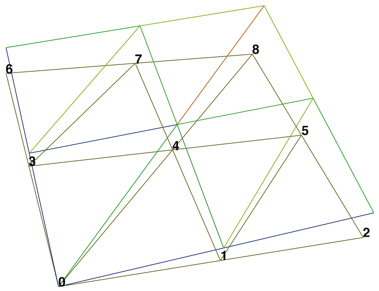
The vertex numbering may be examined by using the FEniCS plot
command. To do this, plot the function u, press w to turn on
wireframe instead of a fully colored surface, m to show the mesh,
and then v to show the numbering of the vertices.
Let’s instead examine the values by calling
u.compute_vertex_values:
>>> vertex_values = u.compute_vertex_values()
>>> for i, x in enumerate(coordinates):
...     print('vertex %d: vertex_values[%d] = %g\tu(%s) = %g' %
...           (i, i, vertex_values[i], x, u(x)))
vertex 0: vertex_values[0] = 0          u([ 0.  0.]) = 8.46545e-16
vertex 1: vertex_values[1] = 0.5        u([ 0.5  0. ]) = 0.5
vertex 2: vertex_values[2] = 1          u([ 1.  0.]) = 1
vertex 3: vertex_values[3] = 0.5        u([ 0.   0.5]) = 0.5
vertex 4: vertex_values[4] = 1          u([ 0.5  0.5]) = 1
vertex 5: vertex_values[5] = 1.5        u([ 1.   0.5]) = 1.5
vertex 6: vertex_values[6] = 1          u([ 0.  1.]) = 1
vertex 7: vertex_values[7] = 1.5        u([ 0.5  1. ]) = 1.5
vertex 8: vertex_values[8] = 2          u([ 1.  1.]) = 2
We can ask FEniCS to give us the mapping from vertices to degrees of freedom for a certain function space \(V\):
v2d = vertex_to_dof_map(V)
Now, nodal_values[v2d[i]] will give us the value of the degree of
freedom
corresponding to vertex i (v2d[i]). In particular, nodal_values[v2d]
is an array with all the elements in the same (vertex numbered) order
as coordinates. The inverse map, from degrees of freedom number to
vertex number is given by dof_to_vertex_map(V). This means that
we may call
coordinates[dof_to_vertex_map(V)] to get an array of all the
coordinates in the same order as the degrees of freedom. Note that
these mappings are only available in FEniCS for \(\mathsf{P}_1\) elements.
For Lagrange elements of degree larger than 1, there are degrees of
freedom (nodes) that do not correspond to vertices. For these
elements, we may get the vertex values by calling
u.compute_vertex_values(mesh), and we can get the degrees of freedom
by the call u.vector().array(). To get the coordinates associated
with all degrees of freedom, we need to iterate over the elements of
the mesh and ask FEniCS to return the coordinates and dofs associated
with each element (cell). This information is stored in the
FiniteElement and DofMap object of a FunctionSpace. The
following code illustrates how to iterate over all elements of a mesh
and print the coordinates and degrees of freedom associated with the
element.
element = V.element()
dofmap = V.dofmap()
for cell in cells(mesh):
    print(element.tabulate_dof_coordinates(cell))
    print(dofmap.cell_dofs(cell.index()))
We have seen how to extract the nodal values in a numpy array.
If desired, we can adjust the nodal values too. Say we want to
normalize the solution such that \(\max_j |U_j| = 1\). Then we
must divide all \(U_j\) values
by \(\max_j |U_j|\). The following function performs the task:
def normalize_solution(u):
    "Normalize u: return u divided by max(u)"
    u_array = u.vector().array()
    u_max = np.max(np.abs(u_array))
    u_array /= u_max
    u.vector()[:] = u_array
    #u.vector().set_local(u_array)  # alternative
    return u
When using Lagrange elements, this (approximately) ensures that the maximum value of the function \(u\) is \(1\).
The /= operator implies an
in-place modification of the object on the left-hand side: all
elements of the array nodal_values are divided by the value u_max.
Alternatively, we could do nodal_values = nodal_values / u_max, which
implies creating a new array on the right-hand side and assigning this
array to the name nodal_values.
Be careful when manipulating degrees of freedom
A call like u.vector().array() returns a copy of the data in
u.vector(). One must therefore never perform assignments like
u.vector.array()[:] = ..., but instead extract the numpy array
(i.e., a copy), manipulate it, and insert it back with u.vector()[:]
= `` or use ``u.set_local(...).
A FEniCS Function object is uniquely defined in the interior
of each cell of the finite element mesh. For continuous (Lagrange)
function spaces, the function values are also uniquely defined on
cell boundaries. A Function object u can be evaluated by simply
calling
u(x)
where x is either a Point or a Python tuple of the correct space
dimension. When a Function is evaluated, FEniCS must first find
which cell of the mesh that contains the given point (if any), and
then evaluate a linear combination of basis functions at the given
point inside the cell in question. FEniCS uses efficient data
structures (bounding box trees) to quickly find the point, but
building the tree is a relatively expensive operation so the cost of
evaluating a Function at a single point is costly. Repeated
evaluation will reuse the computed data structures and thus be
relatively less expensive.
Cheap vs expensive function evaluation
A Function object u can be evaluated in various ways:
u(x) for an arbitrary point xu.vector().array()[i] for degree of freedom number iu.compute_vertex_values()[i] at vertex number iThe first method, though very flexible, is in general expensive while the other two are very efficient (but limited to certain points).
To demonstrate the use of point evaluation of Function objects, we
print the value of the computed finite element solution u for the
Poisson problem at the center point of the domain and compare it with
the exact solution:
center = (0.5, 0.5)
error = u_D(center) - u(center)
print('Error at %s: %g' % (center, error))
For a \(2\times(3\times 3)\) mesh, the output from the previous snippet becomes
Error at (0.5, 0.5): -0.0833333
The discrepancy is due to the fact that the center point is not a node
in this particular mesh, but a point in the interior of a cell, and
u varies linearly over the cell while u_D is a quadratic
function. When the center point is a node, as in a \(2\times(2\times
2)\) or \(2\times(4\times 4)\) mesh, the error is of the order
\(10^{-15}\).
As the final theme in this chapter, we will look at how to postprocess computations; that is, how to compute various derived quantities from the computed solution of a PDE. The solution \(u\) itself may be of interest for visualizing general features of the solution, but sometimes one is interested in computing the solution of a PDE to compute a specific quantity that derives from the solution, such as, e.g., the flux, a point-value, or some average of the solution.
As a test problem, we consider again the variable-coefficient Poisson problem with a single Dirichlet boundary condition:
Let us continue to use our favorite solution \(u(x,y)=1+x^2+2y^2\) and then prescribe \(\kappa(x,y)=x+y\). It follows that \(u_{_\mathrm{D}}(x,y) = 1 + x^2 + 2y^2\) and \(f(x,y)=-8x-10y\).
As before, the variational formulation for this model problem can be specified in FEniCS as
a = kappa*dot(grad(u), grad(v))*dx
L = f*v*dx
with the coefficient \(\kappa\) and right-hand side \(f\) given by
kappa = Expression('x[0] + x[1]', degree=1)
f = Expression('-8*x[0] - 10*x[1]', degree=1)
It is often of interest to compute the flux \(Q = -\kappa\nabla u\). Since \(u = \sum_{j=1}^N U_j \phi_j\), it follows that
We note that the gradient of a piecewise continuous finite element scalar field is a discontinuous vector field since the basis functions \(\{\phi_j\}\) have discontinuous derivatives at the boundaries of the cells. For example, using Lagrange elements of degree 1, \(u\) is linear over each cell, and the gradient becomes a piecewise constant vector field. On the contrary, the exact gradient is continuous. For visualization and data analysis purposes, we often want the computed gradient to be a continuous vector field. Typically, we want each component of \(\nabla u\) to be represented in the same way as \(u\) itself. To this end, we can project the components of \(\nabla u\) onto the same function space as we used for \(u\). This means that we solve \(w = \nabla u\) approximately by a finite element method, using the same elements for the components of \(w\) as we used for \(u\). This process is known as projection.
Projection is a common operation in finite element analysis and, as
we have already seen, FEniCS
has a function for easily performing the projection:
project(expression, W), which returns the projection of some
expression into the space W.
In our case, the flux \(Q = -\kappa\nabla u\)
is vector-valued and we need to pick W as the vector-valued function
space of the same degree as the space V where u resides:
V = u.function_space()
mesh = V.mesh()
degree = V.ufl_element().degree()
W = VectorFunctionSpace(mesh, 'P', degree)

grad_u = project(grad(u), W)
flux_u = project(-k*grad(u), W)
The applications of projection are many, including turning discontinuous gradient fields into continuous ones, comparing higher- and lower-order function approximations, and transforming a higher-order finite element solution down to a piecewise linear field, which is required by many visualization packages.
Plotting the flux vector field is naturally as easy as plotting anything else:
plot(flux_u, title='flux field')

flux_x, flux_y = flux_u.split(deepcopy=True)  # extract components
plot(flux_x, title='x-component of flux (-kappa*grad(u))')
plot(flux_y, title='y-component of flux (-kappa*grad(u))')
The deepcopy=True argument signifies a deep copy, which is
a general term in computer science implying that a copy of the data is
returned. (The opposite, deepcopy=False,
means a shallow copy, where
the returned objects are just pointers to the original data.)
For data analysis of the nodal values of the flux field, we can
grab the underlying numpy arrays (which demands a deepcopy=True
in the split of flux):
flux_x_nodal_values = flux_x.vector().dofs()
flux_y_nodal_values = flux_y.vector().dofs()
The degrees of freedom of the flux_u vector field can also be
reached by
flux_u_nodal_values = flux_u.vector().array()
However, this is a flat numpy array containing the degrees of
freedom for both the \(x\) and \(y\) components of the flux and the
ordering of the components may be mixed up by FEniCS in order to
improve computational efficiency.
The function demo_flux in the program
ft10_poisson_extended.py
demonstrates the computations described above.
Manual projection
Although you will always use project to project a finite element
function, it can be instructive to look at how to formulate the
projection mathematically and implement its steps manually in FEniCS.
Let’s say we have an expression \(g = g(u)\) that we want to project into some space \(W\). The mathematical formulation of the (\(L^2\)) projection \(w = P_W g\) into \(W\) is the variational problem
After the solution \(u\) of a PDE is computed, we occasionally want to compute functionals of \(u\), for example,
which often reflects some energy quantity. Another frequently occurring functional is the error
where \({u_{\small\mbox{e}}}\) is the exact solution. The error is of particular interest when studying convergence properties of finite element methods. Other times, we may instead be interested in computing the flux out through a part \(\Gamma\) of the boundary \(\partial\Omega\),
where \(n\) is the outward-pointing unit normal on \(\Gamma\).
All these functionals are easy to compute with FEniCS, as we shall see in the examples below.
The integrand of the energy functional (94) is described in the UFL language in the same manner as we describe weak forms:
energy = 0.5*dot(grad(u), grad(u))*dx
E = assemble(energy)
The functional energy is evaluated by calling the assemble
function that we have previously used to assemble matrices and
vectors. FEniCS will recognize that the form has ‘’rank 0’’ (since it
contains no trial and test functions) and return the result as a
scalar value.
The functional (95) can be computed as follows:
error = (u_e - u)**2*dx
E = sqrt(abs(assemble(error)))
The exact solution \({u_{\small\mbox{e}}}\) is here represented by a Function or
Expression object u_e, while u is the finite element
approximation (and thus a Function). Sometimes, for very small
error values, the result of assemble(error) can be a (very small)
negative number, so we have used abs in the expression for E above
to ensure a positive value for the sqrt function.
As will be explained and demonstrated in the section Computing convergence rates, the integration of (u_e - u)**2*dx
can result in too optimistic convergence rates unless one is careful
how the difference u_e - u is evaluated. The general recommendation
for reliable error computation is to use the errornorm function:
E = errornorm(u_e, u)
To compute flux integrals like \(F = -\int_\Gamma \kappa\nabla u\cdot n {\, \mathrm{d}s}\), we need to define the \(n\) vector, referred to as a facet normal in FEniCS. If the surface domain \(\Gamma\) in the flux integral is the complete boundary, we can perform the flux computation by
n = FacetNormal(mesh)
flux = -k*dot(grad(u), n)*ds
total_flux = assemble(flux)
Although grad(u) and nabla_grad(u) are interchangeable in the above
expression when u is a scalar function, we have chosen to write
grad(u) because this is the right expression if we generalize the
underlying equation to a vector PDE. With nabla_grad(u) we
must in that case write dot(n, nabla_grad(u)).
It is possible to restrict the integration to a part of the boundary
by using a mesh function to mark the relevant part, as explained in
the section Setting multiple Dirichlet, Neumann, and Robin conditions. Assuming that the part corresponds
to subdomain number i, the relevant syntax for the variational
formulation of the flux is -k*dot(grad(u), n)*ds(i).
A note on the accuracy of integration
As we have seen before, FEniCS Expressions must be defined using
a particular degree. The degree tells FEniCS into which local
finite element space the expression should be interpolated when
performing local computations (integration). As an illustration,
consider the computation of the integral \(\int_0^1 \cos x {\, \mathrm{d}x} = \sin
1\). This may be computed in FEniCS by
mesh = UnitIntervalMesh(1)
I = assemble(Expression('cos(x[0])', degree=degree)*dx(domain=mesh))
Note that we must here specify the argument domain=mesh to the
measure dx. This is normally not necessary when defining forms
in FEniCS but is necessary here since cos(x[0]) is not associated
with any domain (as is the case when we integrate a Function
from some FunctionSpace defined on some Mesh).
Varying the degree between 0 and 5, the value of \(|\sin(1) - I|\) is
0.036,
0.071,
0.00030,
0.00013,
4.5E-07, and
2.5E-07.
FEniCS also allows expressions to be expressed directly as part of
a form. This requires the creation of a SpatialCoordinate.
In this case, the accuracy is dictated by the accuracy of the
integration, which may be controlled by a degree argument to
the integration measure dx. The degree argument specifies
that the integration should be exact for polynomials of that degree.
The following code snippet shows how to compute the integral \(\int_0^1 \cos x {\, \mathrm{d}x}\) using this approach:
mesh = UnitIntervalMesh(1)
x = SpatialCoordinate(mesh)
I = assemble(cos(x[0])*dx(degree=degree))
Varying the degree between 0 and 5, the value of \(|\sin(1) - I|\) is
0.036,
0.036,
0.00020,
0.00020,
4.3E-07,
4.3E-07.
Note that the quadrature degrees are only available for
odd degrees so that degree \(0\) will use the same quadrature
rule as degree \(1\),
degree \(2\) will give the same quadrature rule as degree \(3\) and so on.
A central question for any numerical method is its convergence rate: how fast does the error approach zero when the resolution is increased? For finite element methods, this typically corresponds to proving, theoretically or empirically, that the error \(e = {u_{\small\mbox{e}}} - u\) is bounded by the mesh size \(h\) to some power \(r\); that is, \(\|e\| \leq C h^r\) for some constant \(C\). The number \(r\) is called the convergence rate of the method. Note that different norms, like the \(L^2\)-norm \(\|e\|\) or \(H^1_0\)-norm \(\|\nabla e\|\) typically have different convergence rates.
To illustrate how to compute errors and convergence rates in FEniCS,
we have included the function compute_convergence_rates in the
tutorial program
ft10_poisson_extended.py.
This is a tool that is very handy when verifying finite element codes
and will therefore be explained in detail here.
As we have already seen, the \(L^2\)-norm of the error \({u_{\small\mbox{e}}} - u\) can be implemented in FEniCS by
error = (u_e - u)**2*dx
E = sqrt(abs(assemble(error)))
As above, we have used abs in the expression for E above to ensure
a positive value for the sqrt function.
It is important to understand how FEniCS computes the error from the
above code, since we may otherwise run into subtle issues when using
the value for computing convergence rates. The first subtle issue is
that if u_e is not already a finite element function (an object created
using Function(V)), which is the case if u_e is defined as an
Expression, FEniCS must interpolate u_e into some local finite
element space on each element of the mesh. The degree used for the
interpolation is determined by the mandatory keyword argument to the
Expression class, for example:
u_e = Expression('sin(x[0])', degree=1)
This means that the error computed will not be equal to the actual error \(\|{u_{\small\mbox{e}}} - u\|\) but rather the difference between the finite element solution \(u\) and the piecewise linear interpolant of \({u_{\small\mbox{e}}}\). This may yield a too optimistic (too small) value for the error. A better value may be achieved by interpolating the exact solution into a higher-order function space, which can be done by simply increasing the degree:
u_e = Expression('sin(x[0])', degree=3)
The second subtle issue is that when FEniCS evaluates the expression
(u_e - u)**2, this will be expanded into u_e**2 + u**2 -
2*u_e*u. If the error is small (and the solution itself is of
moderate size), this calculation will correspond to the subtraction of
two positive numbers (u_e**2 + u**2 \(\sim 1\) and 2*u_e*u \(\sim
1\)) yielding a small number. Such a computation is very prone to
round-off errors, which may again lead to an unreliable value for the
error. To make this situation worse, FEniCS may expand this
computation into a large number of terms, in particular for higher
order elements, making the computation very unstable.
To help with these issues, FEniCS provides the built-in function
errornorm which computes the error norm in a more intelligent
way. First, both u_e and u are interpolated into a higher-order
function space. Then, the degrees of freedom of u_e and u are
subtracted to produce a new function in the higher-order function
space. Finally, FEniCS integrates the square of the difference
function and then takes the square root to get the value of the error
norm. Using the errornorm function is simple:
E = errornorm(u_e, u, normtype='L2')
It is illustrative to look at a short implementation of errornorm:
def errornorm(u_e, u):
    V = u.function_space()
    mesh = V.mesh()
    degree = V.ufl_element().degree()
    W = FunctionSpace(mesh, 'P', degree + 3)
    u_e_W = interpolate(u_e, W)
    u_W = interpolate(u, W)
    e_W = Function(W)
    e_W.vector()[:] = u_e_W.vector().array() - u_W.vector().array()
    error = e_W**2*dx
    return sqrt(abs(assemble(error)))
Sometimes it is of interest to compute the error of the
gradient field: \(||\nabla ({u_{\small\mbox{e}}}-u)||\),
often referred to as the \(H^1_0\) or \(H^1\) seminorm of the error.
This can either be expressed as above, replacing the expression for
error by error = dot(grad(e_W), grad(e_W))*dx, or by calling
errornorm in FEniCS:
E = errornorm(u_e, u, norm_type='H10')
Type help(errornorm) in Python for more information about available
norm types.
The function compute_errors in
ft10_poisson_extended.py
illustrates the computation of various error norms in FEniCS.
Let’s examine how to compute convergence rates in FEniCS.
The solver function in
ft10_poisson_extended.py
allows us to easily compute solutions for finer and finer meshes and
enables us to study the convergence rate. Define the element size
\(h=1/n\), where \(n\) is the number of cell divisions in the \(x\) and \(y\)
directions (n = Nx = Ny in the code). We perform experiments with
\(h_0>h_1>h_2>\cdots\) and compute the corresponding errors \(E_0, E_1,
E_2\) and so forth. Assuming \(E_i=Ch_i^r\) for unknown constants \(C\) and
\(r\), we can compare two consecutive experiments, \(E_{i-1}=Ch_{i-1}^r\)
and \(E_i=Ch_i^r\), and solve for \(r\):
The \(r\) values should approach the expected convergence rate (typically the polynomial degree + 1 for the \(L^2\)-error) as \(i\) increases.
The procedure above can easily be turned into Python code. Here
we run through a list of element degrees (\(\mathsf{P}_1\),
\(\mathsf{P}_2\), and \(\mathsf{P}_3\)),
perform experiments over a series of refined meshes, and for
each experiment report the six error types as returned by compute_errors.
To demonstrate the computation of convergence rates, we pick an exact solution \({u_{\small\mbox{e}}}\), this time a little more interesting than for the test problem in the chapter Fundamentals: Solving the Poisson equation:
This choice implies \(f(x,y)=2\omega^2\pi^2 u(x,y)\). With \(\omega\) restricted to an integer, it follows that the boundary value is given by \(u_{_\mathrm{D}}=0\).
We need to define the appropriate boundary conditions, the exact solution, and the \(f\) function in the code:
def boundary(x, on_boundary):
    return on_boundary

bc = DirichletBC(V, Constant(0), boundary)

omega = 1.0
u_e = Expression('sin(omega*pi*x[0])*sin(omega*pi*x[1])',
                 degree=6, omega=omega)

f = 2*pi**2*omega**2*u_e
An implementation of the computation of the convergence rate can be
found in the function demo_convergence_rates in the demo program
ft10_poisson_extended.py.
We achieve some interesting results.
Using the infinity norm of the difference of the degrees of freedom,
we obtain the following table:
| element | :math:`n=8` | :math:`n=16` | :math:`n=32` | :math:`n=64` |
|---|---|---|---|---|
| \(\mathsf{P}_1\) | 1.99 | 2.00 | 2.00 | 2.00 |
| \(\mathsf{P}_2\) | 3.99 | 4.00 | 4.00 | 4.01 |
| \(\mathsf{P}_3\) | 3.95 | 3.99 | 3.99 | 3.92 |
An entry like 3.99 for \(n=32\) and \(\mathsf{P}_3\) means that we estimate the rate 3.99 by comparing two meshes, with resolutions \(n=32\) and \(n=16\), using \(\mathsf{P}_3\) elements. Note the superconvergence for \(\mathsf{P}_2\) at the nodes. The best estimates of the rates appear in the right-most column, since these rates are based on the finest resolutions and are hence deepest into the asymptotic regime (until we reach a level where round-off errors and inexact solution of the linear system starts to play a role).
The \(L^2\)-norm errors computed using the FEniCS
errornorm function show the
expected \(h^{d+1}\) rate for \(u\):
| element | :math:`n=8` | :math:`n=16` | :math:`n=32` | :math:`n=64` |
|---|---|---|---|---|
| \(\mathsf{P}_1\) | 1.97 | 1.99 | 2.00 | 2.00 |
| \(\mathsf{P}_2\) | 3.00 | 3.00 | 3.00 | 3.00 |
| \(\mathsf{P}_3\) | 4.04 | 4.02 | 4.01 | 4.00 |
However, using (u_e - u)**2 for the error computation, with the same
degree for the interpolation of u_e as for u, gives strange
results:
| element | :math:`n=8` | :math:`n=16` | :math:`n=32` | :math:`n=64` |
|---|---|---|---|---|
| \(\mathsf{P}_1\) | 1.97 | 1.99 | 2.00 | 2.00 |
| \(\mathsf{P}_2\) | 3.00 | 3.00 | 3.00 | 3.01 |
| \(\mathsf{P}_3\) | 4.04 | 4.07 | 1.91 | 0.00 |
This is an example where it is important to interpolate u_e to a
higher-order space (polynomials of degree 3 are sufficient here). This
is handled automatically by using the errornorm function.
Checking convergence rates is an excellent method for verifying PDE codes.
Many readers have extensive experience with visualization and data analysis of 1D, 2D, and 3D scalar and vector fields on uniform, structured meshes, while FEniCS solvers exclusively work with unstructured meshes. Since it can many times be practical to work with structured data, we discuss in this section how to extract structured data for finite element solutions computed with FEniCS.
A necessary first step is to transform our Mesh object to an object
representing a rectangle (or a 3D box) with equally-shaped
rectangular cells. The second step is to transform the
one-dimensional array of nodal values to a two-dimensional array
holding the values at the corners of the cells in the structured
mesh. We want to access a value by its \(i\) and \(j\) indices, \(i\)
counting cells in the \(x\) direction, and \(j\) counting cells in the \(y\)
direction. This transformation is in principle straightforward, yet
it frequently leads to obscure indexing errors, so using software
tools to ease the work is advantageous.
In the directory of example programs included with this book, we have
included the Python module
boxfield
which provides utilities for working with structured mesh data in
FEniCS. Given a finite element function u, the following function
returns a BoxField object that represents u on a structured mesh:
from boxfield import *
u_box = FEniCSBoxField(u, (nx, ny))
The u_box object contains several useful data structures:
u_box.grid: object for the structured meshu_box.grid.coor[X]: grid coordinates inX=0directionu_box.grid.coor[Y]: grid coordinates inY=1directionu_box.grid.coor[Z]: grid coordinates inZ=2directionu_box.grid.coorv[X]: vectorized version ofu_box.grid.coor[X]u_box.grid.coorv[Y]: vectorized version ofu_box.grid.coor[Y]u_box.grid.coorv[Z]: vectorized version ofu_box.grid.coor[Z]u_box.values:numpyarray holding theuvalues;u_box.values[i,j]holdsuat the mesh point with coordinates
(u_box.grid.coor[X][i], u_box.grid.coor[Y][j])Let us now use the solver function from the
ft10_poisson_extended.py
code to compute u, map it onto a BoxField object for a structured
mesh representation, and print the coordinates and function values
at all mesh points:
u = solver(p, f, u_b, nx, ny, 1, linear_solver='direct')
u_box = structured_mesh(u, (nx, ny))
u_ = u_box.values

# Iterate over 2D mesh points (i, j)
for j in range(u_.shape[1]):
    for i in range(u_.shape[0]):
        print('u[%d, %d] = u(%g, %g) = %g' %
              (i, j,
               u_box.grid.coor[X][i], u_box.grid.coor[Y][j],
               u_[i, j]))
Using the multidimensional array u_ = u_box.values, we can easily
express finite difference approximations of derivatives:
x = u_box.grid.coor[X]
dx = x[1] - x[0]
u_xx = (u_[i - 1, j] - 2*u_[i, j] + u_[i + 1, j]) / dx**2
The ability to access a finite element field as structured data is handy in many occasions, e.g., for visualization and data analysis. Using Matplotlib, we can create a surface plot, as shown in Figure Various plots of the solution on a structured mesh (upper left):
import matplotlib.pyplot as plt
from mpl_toolkits.mplot3d import Axes3D  # necessary for 3D plotting
from matplotlib import cm
fig = plt.figure()
ax = fig.gca(projection='3d')
cv = u_box.grid.coorv  # vectorized mesh coordinates
ax.plot_surface(cv[X], cv[Y], u_, cmap=cm.coolwarm,
                rstride=1, cstride=1)
plt.title('Surface plot of solution')
The key issue is to know that the coordinates needed for the surface
plot is in u_box.grid.coorv and that the values are in u_.
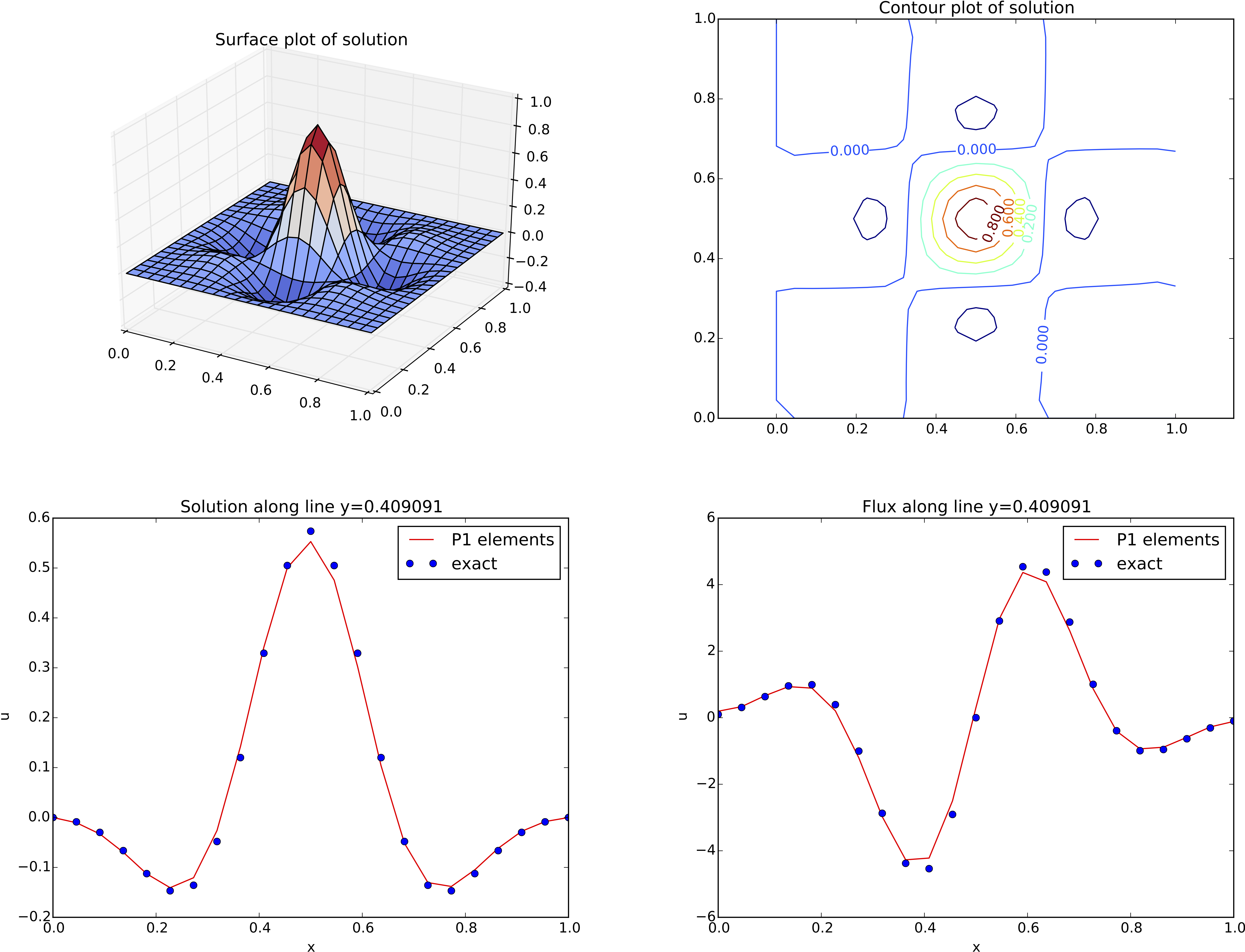
Various plots of the solution on a structured mesh
A contour plot can also be made by Matplotlib:
fig = plt.figure()
ax = fig.gca()
levels = [1.5, 2.0, 2.5, 3.5]
cs = ax.contour(cv[X], cv[Y], u_, levels=levels)
plt.clabel(cs)  # add labels to contour lines
plt.axis('equal')
plt.title('Contour plot of solution')
The result appears in Figure Various plots of the solution on a structured mesh (upper right).
A handy feature of BoxField objects is the ability to give a starting
point in the domain and a direction, and then extract the field and
corresponding coordinates along the nearest line of mesh points. We have
already seen how to interpolate the solution along a line in the mesh, but
with BoxField you can pick out the computational points (vertices) for
examination of these points. Numerical methods often show improved behavior
at such points so this is of interest. For 3D fields
one can also extract data in a plane.
Say we want to plot \(u\) along
the line \(y=0.4\). The mesh points, x, and the \(u\) values
along this line, u_val, can be extracted by
start = (0, 0.4)
x, u_val, y_fixed, snapped = u_box.gridline(start, direction=X)
The variable snapped is true if the line is snapped onto to nearest
gridline and in that case y_fixed holds the snapped
(altered) \(y\) value. The keyword argument snap is by default True
to avoid interpolation and force snapping.
A comparison of the numerical and exact solution along the line \(y\approx 0.41\) (snapped from \(y=0.4\)) is made by the following code:
# Plot u along a line y = const and compare with exact solution
start = (0, 0.4)
x, u_val, y_fixed, snapped = u_box.gridline(start, direction=X)
u_e_val = [u_D((x_, y_fixed)) for x_ in x]
plt.figure()
plt.plot(x, u_val, 'r-')
plt.plot(x, u_e_val, 'bo')
plt.legend(['P1 elements', 'exact'], loc='best')
plt.title('Solution along line y=%g' % y_fixed)
plt.xlabel('x');  plt.ylabel('u')
See Figure Various plots of the solution on a structured mesh (lower left) for the resulting curve plot.
Let us also compare the numerical and exact fluxes \(-\kappa\partial u/\partial x\) along the same line as above:
# Plot the numerical and exact flux along the same line
flux_u = flux(u, kappa)
flux_u_x, flux_u_y = flux_u.split(deepcopy=True)
flux2_x = flux_u_x if flux_u_x.ufl_element().degree() == 1 \
          else interpolate(flux_x,
               FunctionSpace(u.function_space().mesh(), 'P', 1))
flux_u_x_box = FEniCSBoxField(flux_u_x, (nx,ny))
x, flux_u_val, y_fixed, snapped = \
   flux_u_x_box.gridline(start, direction=X)
y = y_fixed
plt.figure()
plt.plot(x, flux_u_val, 'r-')
plt.plot(x, flux_u_x_exact(x, y_fixed), 'bo')
plt.legend(['P1 elements', 'exact'], loc='best')
plt.title('Flux along line y=%g' % y_fixed)
plt.xlabel('x');  plt.ylabel('u')
The function flux called at the beginning of the code snippet is
defined in the example program
ft10_poisson_extended.py
and interpolates the flux back into the function space.
Note that Matplotlib is one choice of plotting package. With the unified interface in the SciTools package one can access Matplotlib, Gnuplot, MATLAB, OpenDX, VisIt, and other plotting engines through the same API.
The graphics referred to in Figure Various plots of the solution on a structured mesh correspond to a test problem with prescribed solution \({u_{\small\mbox{e}}} = H(x)H(y)\), where
The corresponding right-hand side \(f\) is obtained by inserting the exact
solution into the PDE and differentiating as before.
Although it is easy to carry out the
differentiation of \(f\) by hand and hardcode the resulting expressions
in an Expression object, a more reliable habit is to use Python’s
symbolic computing engine, SymPy, to perform mathematics and
automatically turn formulas into C++ syntax for Expression objects.
A short introduction was given in
the section FEniCS implementation (5).
We start out with defining the exact solution in sympy:
from sympy import exp, sin, pi  # for use in math formulas
import sympy as sym

H = lambda x: exp(-16*(x-0.5)**2)*sin(3*pi*x)
x, y = sym.symbols('x[0], x[1]')
u = H(x)*H(y)
Turning the expression for u into C or C++ syntax for Expression objects
needs two steps. First we ask for the C code of the expression:
u_code = sym.printing.ccode(u)
Printing u_code gives (the output is here manually broken into two
lines):
-exp(-16*pow(x[0] - 0.5, 2) - 16*pow(x[1] - 0.5, 2))*
sin(3*M_PI*x[0])*sin(3*M_PI*x[1])
The necessary syntax adjustment is replacing
the symbol M_PI for \(\pi\) in C/C++ by pi (or DOLFIN_PI):
u_code = u_code.replace('M_PI', 'pi')
u_b = Expression(u_code, degree=1)
Thereafter, we can progress with the computation of \(f = -\nabla\cdot(\kappa\nabla u)\):
kappa = 1
f = sym.diff(-kappa*sym.diff(u, x), x) + \
    sym.diff(-kappa*sym.diff(u, y), y)
f = sym.simplify(f)
f_code = sym.printing.ccode(f)
f_code = f_code.replace('M_PI', 'pi')
f = Expression(f_code, degree=1)
We also need a Python function for the exact flux \(-\kappa\partial u/\partial x\):
flux_u_x_exact = sym.lambdify([x, y], -kappa*sym.diff(u, x),
                              modules='numpy')
It remains to define kappa = Constant(1) and set nx and ny before calling
solver to compute the finite element solution of this problem.
If you have come this far, you have learned how to both write simple script-like solvers for a range of PDEs, and how to structure Python solvers using functions and unit tests. Solving a more complex PDE and writing a more full-featured PDE solver is not much harder and the first step is typically to write a solver for a stripped-down test case as a simple Python script. As the script matures and becomes more complex, it is time to think about design, in particular how to modularize the code and organize it into reusable pieces that can be used to build a flexible and extensible solver.
On the FEniCS web site you will find more extensive documentation, more example programs, and links to advanced solvers and applications written on top of FEniCS. Get inspired and develop your own solver for your favorite application, publish your code and share your knowledge with the FEniCS community and the world!
PS: Stay tuned for the FEniCS Tutorial Volume 2!
| [Ref01] | A. Logg, K.-A. Mardal and G. N. Wells. Automated Solution of Partial Differential Equations by the Finite Element Method, Springer, 2012. |
| [Ref02] | A. Logg and G. N. Wells. DOLFIN: Automated Finite Element Computing, ACM Transactions on Mathematical Software, 37(2), doi: 10.1145/1731022.1731030, arXiv: 1103.6248, 2010, http://www.dspace.cam.ac.uk/handle/1810/221918/. |
| [Ref03] | R. C. Kirby and A. Logg. A Compiler for Variational Forms, ACM Transactions on Mathematical Software, 32(3), pp. 417-444, doi: 10.1145/1163641.1163644, arXiv: 1112.0402, 2006. |
| [Ref04] | R. C. Kirby. FIAT, a new paradigm for computing finite element basis functions, ACM Transactions on Mathematical Software, 30(4), pp. 502-516, 2004. |
| [Ref05] | M. S. Alnæs, A. Logg, K. B. Ølgaard, M. E. Rognes and G. N. Wells. Unified Form Language: A domain-specific language for weak formulations of partial differential equations, ACM Transactions on Mathematical Software, 40(2), 2014, doi:10.1145/2566630, arXiv:1211.4047. |
| [Ref06] | P. S. Foundation. The Python Tutorial, http://docs.python.org/2/tutorial. |
| [Ref07] | H. P. Langtangen and L. R. Hellevik. Brief Tutorials on Scientific Python, 2016, http://hplgit.github.io/bumpy/doc/web/index.html. |
| [Ref08] | M. Pilgrim. Dive into Python, Apress, 2004, http://www.diveintopython.net. |
| [Ref09] | H. P. Langtangen. Python Scripting for Computational Science, third edition, Springer, 2009. |
| [Ref10] | H. P. Langtangen. A Primer on Scientific Programming With Python, fifth edition, Texts in Computational Science and Engineering, Springer, 2016. |
| [Ref11] | J. M. Kinder and P. Nelson. A Student’s Guide to Python for Physical Modeling, Princeton University Press, 2015. |
| [Ref12] | J. Kiusalaas. Numerical Methods in Engineering With Python, Cambridge University Press, 2005. |
| [Ref13] | R. H. Landau, M. J. Paez and C. C. Bordeianu. Computational Physics: Problem Solving with Python, third edition, Wiley, 2015. |
| [Ref14] | H. P. Langtangen and K.-A. Mardal. Introduction to Numerical Methods for Variational Problems, 2016, http://hplgit.github.io/fem-book/doc/web/. |
| [Ref15] | M. G. Larson and F. Bengzon. The Finite Element Method: Theory, Implementation, and Applications, Texts in Computational Science and Engineering, Springer, 2013. |
| [Ref16] | M. Gockenbach. Understanding and Implementing the Finite Element Method, SIAM, 2006. |
| [Ref17] | J. Donea and A. Huerta. Finite Element Methods for Flow Problems, Wiley Press, 2003. |
| [Ref18] | T. J. R. Hughes. The Finite Element Method: Linear Static and Dynamic Finite Element Analysis, Prentice-Hall, 1987. |
| [Ref19] | W. B. Bickford. A First Course in the Finite Element Method, 2nd edition, Irwin, 1994. |
| [Ref20] | K. Eriksson, D. Estep, P. Hansbo and C. Johnson. Computational Differential Equations, Cambridge University Press, 1996. |
| [Ref21] | S. C. Brenner and L. R. Scott. The Mathematical Theory of Finite Element Methods, third edition, Texts in Applied Mathematics, Springer, 2008. |
| [Ref22] | D. Braess. Finite Elements, third edition, Cambridge University Press, 2007. |
| [Ref23] | A. Ern and J.-L. Guermond. Theory and Practice of Finite Elements, Springer, 2004. |
| [Ref24] | A. Quarteroni and A. Valli. Numerical Approximation of Partial Differential Equations, Springer Series in Computational Mathematics, Springer, 1994. |
| [Ref25] | P. G. Ciarlet. The Finite Element Method for Elliptic Problems, Classics in Applied Mathematics, SIAM, 2002, Reprint of the 1978 original [North-Holland, Amsterdam; MR0520174 (58 #25001)]. |
| [Ref26] | D. N. Arnold and A. Logg. Periodic Table of the Finite Elements, SIAM News, 2014. |
| [Ref27] | A. H. Squillacote. The ParaView Guide, Kitware, 2007, http://www.paraview.org/paraview-guide/. |
| [Ref28] | H. P. Langtangen and A. Logg. Solving PDEs in Hours – The FEniCS Tutorial Volume II, Springer, 2016. |
| [Ref29] | A. J. Chorin. Numerical solution of the Navier-Stokes equations, Math. Comp., 22, pp. 745-762, 1968. |
| [Ref30] | R. Temam. Sur l’approximation de la solution des ‘equations de Navier-Stokes, Arc. Ration. Mech. Anal., 32, pp. 377-385, 1969. |
| [Ref31] | K. Goda. A multistep technique with implicit difference schemes for calculating two- or three-dimensional cavity flows, Journal of Computational Physics, 30(1), pp. 76-95, 1979. |