3. Biharmonic equation
This demo is implemented in a single Python file,
demo_biharmonic.py, which contains both the variational
forms and the solver.
This demo illustrates how to:
- Solve a linear partial differential equation
- Use a discontinuous Galerkin method
- Solve a fourth-order differential equation
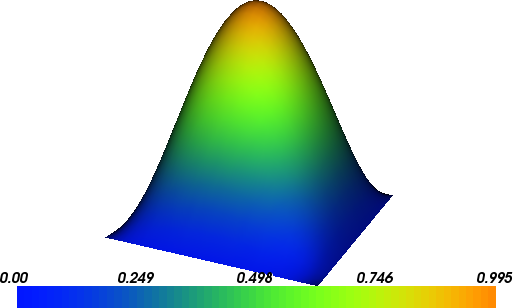
The solution for \(u\) in this demo will look as follows:
3.1. Equation and problem definition
The biharmonic equation is a fourth-order elliptic equation. On the domain \(\Omega \subset \mathbb{R}^{d}\), \(1 \le d \le 3\), it reads
where \(\nabla^{4} \equiv \nabla^{2} \nabla^{2}\) is the biharmonic operator and \(f\) is a prescribed source term. To formulate a complete boundary value problem, the biharmonic equation must be complemented by suitable boundary conditions.
Multiplying the biharmonic equation by a test function and integrating by parts twice leads to a problem second-order derivatives, which would requires \(H^{2}\) conforming (roughly \(C^{0}\) continuous) basis functions. To solve the biharmonic equation using Lagrange finite element basis functions, the biharmonic equation can be split into two second-order equations (see the Mixed Poisson demo for a mixed method for the Poisson equation), or a variational formulation can be constructed that imposes weak continuity of normal derivatives between finite element cells. The demo uses a discontinuous Galerkin approach to impose continuity of the normal derivative weakly.
Consider a triangulation \(\mathcal{T}\) of the domain \(\Omega\), where the union of interior facets is denoted by \(\Gamma\). Functions evaluated on opposite sides of a facet are indicated by the subscripts ‘\(+\)‘ and ‘\(-\)‘. Using the standard continuous Lagrange finite element space
and considering the boundary conditions
a weak formulation of the biharmonic reads: find \(u \in V\) such that
where \(\left< u \right> = (1/2) (u_{+} + u_{-})\), \(\llbracket w \rrbracket = w_{+} \cdot n_{+} + w_{-} \cdot n_{-}\), \(\alpha \ge 0\) is a penalty term and \(h\) is a measure of the cell size. For the implementation, it is useful to identify the bilinear form
and the linear form
The input parameters for this demos are defined as follows:
- \(\Omega = [0,1] \times [0,1]\) (a unit square)
- \(\alpha = 8.0\) (penalty parameter)
- \(f = 4.0 \pi^4\sin(\pi x)\sin(\pi y)\) (source term)
3.2. Implementation
This demo is implemented in the demo_biharmonic.py file.
First, the dolfin module is imported:
from dolfin import *
Next, some parameters for the form compiler are set:
# Optimization options for the form compiler
parameters["form_compiler"]["cpp_optimize"] = True
parameters["form_compiler"]["optimize"] = True
A mesh is created, and a quadratic finite element function space:
# Create mesh and define function space
mesh = UnitSquareMesh(32, 32)
V = FunctionSpace(mesh, "CG", 2)
A subclass of SubDomain,
DirichletBoundary is created for later defining the boundary of
the domian:
# Define Dirichlet boundary
class DirichletBoundary(SubDomain):
    def inside(self, x, on_boundary):
        return on_boundary
A subclass of Expression, Source is created for
the source term \(f\):
class Source(Expression):
    def eval(self, values, x):
        values[0] = 4.0*pi**4*sin(pi*x[0])*sin(pi*x[1])
The Dirichlet boundary condition is created:
# Define boundary condition
u0 = Constant(0.0)
bc = DirichletBC(V, u0, DirichletBoundary())
On the finite element space V, trial and test functions are created:
# Define trial and test functions
u = TrialFunction(V)
v = TestFunction(V)
A function for the cell size \(h\) is created, as is a function
for the average size of cells that share a facet (h_avg). The UFL
syntax ('+') and ('-') restricts a function to the ('+')
and ('-') sides of a facet, respectively. The unit outward normal
to cell boundaries (n) is created, as is the source term f and
the penalty parameter alpha. The penalty parameters is made a
Constant so that it
can be changed without needing to regenerate code.
# Define normal component, mesh size and right-hand side
h = CellSize(mesh)
h_avg = (h('+') + h('-'))/2.0
n = FacetNormal(mesh)
f = Source()

# Penalty parameter
alpha = Constant(8.0)
The bilinear and linear forms are defined:
# Define bilinear form
a = inner(div(grad(u)), div(grad(v)))*dx \
  - inner(avg(div(grad(u))), jump(grad(v), n))*dS \
  - inner(jump(grad(u), n), avg(div(grad(v))))*dS \
  + alpha('+')/h_avg*inner(jump(grad(u),n), jump(grad(v),n))*dS

# Define linear form
L = f*v*dx
A Function is created
to store the solution and the variational problem is solved:
# Solve variational problem
u = Function(V)
solve(a == L, u, bc)
The computed solution is written to a file in VTK format and plotted to the screen.
# Save solution to file
file = File("biharmonic.pvd")
file << u

# Plot solution
plot(u, interactive=True)
3.3. Complete code
from dolfin import *

# Optimization options for the form compiler
parameters["form_compiler"]["cpp_optimize"] = True
parameters["form_compiler"]["optimize"] = True

# Create mesh and define function space
mesh = UnitSquareMesh(32, 32)
V = FunctionSpace(mesh, "CG", 2)

# Define Dirichlet boundary
class DirichletBoundary(SubDomain):
    def inside(self, x, on_boundary):
        return on_boundary

class Source(Expression):
    def eval(self, values, x):
        values[0] = 4.0*pi**4*sin(pi*x[0])*sin(pi*x[1])

# Define boundary condition
u0 = Constant(0.0)
bc = DirichletBC(V, u0, DirichletBoundary())

# Define trial and test functions
u = TrialFunction(V)
v = TestFunction(V)

# Define normal component, mesh size and right-hand side
h = CellSize(mesh)
h_avg = (h('+') + h('-'))/2.0
n = FacetNormal(mesh)
f = Source()

# Penalty parameter
alpha = Constant(8.0)

# Define bilinear form
a = inner(div(grad(u)), div(grad(v)))*dx \
  - inner(avg(div(grad(u))), jump(grad(v), n))*dS \
  - inner(jump(grad(u), n), avg(div(grad(v))))*dS \
  + alpha('+')/h_avg*inner(jump(grad(u),n), jump(grad(v),n))*dS

# Define linear form
L = f*v*dx

# Solve variational problem
u = Function(V)
solve(a == L, u, bc)

# Save solution to file
file = File("biharmonic.pvd")
file << u

# Plot solution
plot(u, interactive=True)