A system of advection–diffusion–reaction equations

The problems we have encountered so far—with the notable exception of the Navier–Stokes equations—all share a common feature: they all involve models expressed by a single scalar or vector PDE. In many situations the model is instead expressed as a system of PDEs, describing different quantities possibly governed by (very) different physics. As we saw for the Navier–Stokes equations, one way to solve a system of PDEs in FEniCS is to use a splitting method where we solve one equation at a time and feed the solution from one equation into the next. However, one of the strengths with FEniCS is the ease by which one can instead define variational problems that couple several PDEs into one compound system. In this section, we will look at how to use FEniCS to write solvers for such systems of coupled PDEs. The goal is to demonstrate how easy it is to implement fully implicit, also known as monolithic, solvers in FEniCS.

PDE problem

Our model problem is the following system of advection–diffusion–reaction equations: $$ \begin{align} \tag{3.37} \frac{\partial u_1}{\partial t} + w \cdot \nabla u_1 - \nabla\cdot(\epsilon\nabla u_1) &= f_1 -K u_1 u_2, \\ \tag{3.38} \frac{\partial u_2}{\partial t} + w \cdot \nabla u_2 - \nabla\cdot(\epsilon\nabla u_2) &= f_2 -K u_1 u_2, \\ \tag{3.39} \frac{\partial u_3}{\partial t} + w \cdot \nabla u_3 - \nabla\cdot(\epsilon\nabla u_3) &= f_3 + K u_1 u_2 - K u_3. \end{align} $$

This system models the chemical reaction between two species $ A $ and $ B $ in some domain $ \Omega $: $$ A + B \rightarrow C. $$

We assume that the reaction is first-order, meaning that the reaction rate is proportional to the concentrations $ [A] $ and $ [B] $ of the two species $ A $ and $ B $: $$ \frac{\mathrm{d}}{\mathrm{d}t} [C] = K [A] [B]. $$ We also assume that the formed species $ C $ spontaneously decays with a rate proportional to the concentration $ [C] $. In the PDE system (3.37)--(3.39), we use the variables $ u_1 $, $ u_2 $, and $ u_3 $ to denote the concentrations of the three species: $$ u_1 = [A], \quad u_2 = [B], \quad u_3 = [C]. $$ We see that the chemical reactions are accounted for in the right-hand sides of the PDE system (3.37)--(3.39).

The chemical reactions take part at each point in the domain $ \Omega $. In addition, we assume that the species $ A $, $ B $, and $ C $ diffuse throughout the domain with diffusivity $ \epsilon $ (the terms $ -\nabla\cdot(\epsilon\nabla u_i) $) and are advected with velocity $ w $ (the terms $ w\cdot\nabla u_i $).

To make things visually and physically interesting, we shall let the chemical reaction take place in the velocity field computed from the solution of the incompressible Navier–Stokes equations around a cylinder from the previous section. In summary, we will thus be solving the following coupled system of nonlinear PDEs: $$ \begin{align} \tag{3.40} \varrho\left(\frac{\partial w}{\partial t} + w \cdot \nabla w\right) &= \nabla\cdot\sigma(w, p) + f, \\ \nabla \cdot w &= 0, \tag{3.41}\\ \frac{\partial u_1}{\partial t} + w \cdot \nabla u_1 - \nabla\cdot(\epsilon\nabla u_1) &= f_1 - K u_1 u_2, \tag{3.42}\\ \frac{\partial u_2}{\partial t} + w \cdot \nabla u_2 - \nabla\cdot(\epsilon\nabla u_2) &= f_2 - K u_1 u_2, \tag{3.43}\\ \frac{\partial u_3}{\partial t} + w \cdot \nabla u_3 - \nabla\cdot(\epsilon\nabla u_3) &= f_3 + K u_1 u_2 - K u_3. \tag{3.44} \end{align} $$ We assume that $ u_1 = u_2 = u_3 = 0 $ at $ t = 0 $ and inject the species $ A $ and $ B $ into the system by specifying nonzero source terms $ f_1 $ and $ f_2 $ close to the corners at the inflow, and take $ f_3 = 0 $. The result will be that $ A $ and $ B $ are convected by advection and diffusion throughout the channel, and when they mix the species $ C $ will be formed.

Since the system is one-way coupled from the Navier–Stokes subsystem to the advection–diffusion–reaction subsystem, we do not need to recompute the solution to the Navier–Stokes equations, but can just read back the previously computed velocity field $ w $ and feed it into our equations. But we do need to learn how to read and write solutions for time-dependent PDE problems.

Variational formulation

We obtain the variational formulation of our system by multiplying each equation by a test function, integrating the second-order terms $ -\nabla\cdot(\epsilon\nabla u_i) $ by parts, and summing up the equations. When working with FEniCS it is convenient to think of the PDE system as a vector of equations. The test functions are collected in a vector too, and the variational formulation is the inner product of the vector PDE and the vector test function.

We also need introduce some discretization in time. We will use the backward Euler method as before when we solved the heat equation and approximate the time derivatives by $ (u_i^{n+1}-u_i^n) / \dt $. Let $ v_1 $, $ v_2 $, and $ v_3 $ be the test functions, or the components of the test vector function. The inner product results in $$ \begin{align} \tag{3.45} & \int_{\Omega} (\dt^{-1} (u_1^{n+1} - u_1^n) v_1 + w \cdot \nabla u^{n+1}_1 \, v_1 + \epsilon \nabla u^{n+1}_1 \cdot \nabla v_1) \dx \\ + & \int_{\Omega} (\dt^{-1} (u_2^{n+1} - u_2^n) v_2 + w \cdot \nabla u^{n+1}_2 \, v_2 + \epsilon \nabla u^{n+1}_2 \cdot \nabla v_2) \dx \nonumber \\ + & \int_{\Omega} (\dt^{-1} (u_3^{n+1} - u_3^n) v_3 + w \cdot \nabla u^{n+1}_3 \, v_3 + \epsilon \nabla u^{n+1}_3 \cdot \nabla v_3) \dx \nonumber \\ - & \int_{\Omega} (f_1 v_1 + f_2 v_2 + f_3 v_3) \dx \nonumber \\ - & \int_{\Omega} (-K u^{n+1}_1 u^{n+1}_2 v_1 - K u^{n+1}_1 u^{n+1}_2 v_2 + K u^{n+1}_1 u^{n+1}_2 v_3 - K u^{n+1}_3 v_3) \dx = 0. \nonumber \end{align} $$ For this problem it is natural to assume homogeneous Neumann boundary conditions on the entire boundary for $ u_1 $, $ u_2 $, and $ u_3 $; that is, $ \partial u_i/\partial n = 0 $ for $ i = 1, 2, 3 $. This means that the boundary terms vanish when we integrate by parts.

FEniCS implementation

The first step is to read the mesh from file. Luckily, we made sure to save the mesh to file in the Navier–Stokes example and can now easily read it back from file:

mesh = Mesh('navier_stokes_cylinder/cylinder.xml.gz')

The mesh is stored in the native FEniCS XML format (with additional gzipping to decrease the file size).

Next, we need to define the finite element function space. For this problem, we need to define several spaces. The first space we create is the space for the velocity field $ w $ from the Navier–Stokes simulation. We call this space $ W $ and define the space by

W = VectorFunctionSpace(mesh, 'P', 2)

It is important that this space is exactly the same as the space we used for the velocity field in the Navier–Stokes solver. To read the values for the velocity field, we use a TimeSeries:

timeseries_w = TimeSeries('navier_stokes_cylinder/velocity_series')

This will initialize the object timeseries_w which we will call later in the time-stepping loop to retrieve values from the file velocity_series.h5 (in binary HDF5 format).

For the three concentrations $ u_1 $, $ u_2 $, and $ u_3 $, we want to create a mixed space with functions that represent the full system $ (u_1, u_2, u_3) $ as a single entity. To do this, we need to define a MixedElement as the product space of three simple finite elements and then used the mixed element to define the function space:

P1 = FiniteElement('P', triangle, 1)
element = MixedElement([P1, P1, P1])
V = FunctionSpace(mesh, element)

Mixed elements as products of elements. FEniCS also allows finite elements to be defined as products of simple elements (or mixed elements). For example, the well-known Taylor–Hood element, with quadratic velocity components and linear pressure functions, may be defined as follows:

P2 = VectorElement('P', triangle, 2)
P1 = FiniteElement('P', triangle, 1)
TH = P2 * P1

This syntax works great for two elements, but for three or more elements we meet a subtle issue in how the Python interpreter handles the * operator. For the reaction system, we create the mixed element by element = MixedElement([P1, P1, P1]) and one would be tempted to write

element = P1 * P1 * P1

However, this is equivalent to writing element = (P1 * P1) * P1 so the result will be a mixed element consisting of two subsystems, the first of which in turn consists of two scalar subsystems.

Finally, we remark that for the simple case of a mixed system consisting of three scalar elements as for the reaction system, the definition is in fact equivalent to using a standard vector-valued element:

element = VectorElement('P', triangle, 1, dim=3)
V = FunctionSpace(mesh, element)

Once the space has been created, we need to define our test functions and finite element functions. Test functions for a mixed function space can be created by replacing TestFunction by TestFunctions:

v_1, v_2, v_3 = TestFunctions(V)

Since the problem is nonlinear, we need to work with functions rather than trial functions for the unknowns. This can be done by using the corresponding Functions construction in FEniCS. However, as we will need to access the Function for the entire system itself, we first need to create that function and then access its components:

u = Function(V)
u_1, u_2, u_3 = split(u)

These functions will be used to represent the unknowns $ u_1 $, $ u_2 $, and $ u_3 $ at the new time level $ n+1 $. The corresponding values at the previous time level $ n $ are denoted by u_n1, u_n2, and u_n3 in our program.

When now all functions and test functions have been defined, we can express the nonlinear variational problem (3.45):

F = ((u_1 - u_n1) / k)*v_1*dx + dot(w, grad(u_1))*v_1*dx \ 
  + eps*dot(grad(u_1), grad(v_1))*dx + K*u_1*u_2*v_1*dx  \ 
  + ((u_2 - u_n2) / k)*v_2*dx + dot(w, grad(u_2))*v_2*dx \ 
  + eps*dot(grad(u_2), grad(v_2))*dx + K*u_1*u_2*v_2*dx  \ 
  + ((u_3 - u_n3) / k)*v_3*dx + dot(w, grad(u_3))*v_3*dx \ 
  + eps*dot(grad(u_3), grad(v_3))*dx - K*u_1*u_2*v_3*dx + K*u_3*v_3*dx \ 
  - f_1*v_1*dx - f_2*v_2*dx - f_3*v_3*dx

The time-stepping simply consists of solving this variational problem in each time step by a call to the solve function:

t = 0
for n in range(num_steps):
    t += dt
    timeseries_w.retrieve(w.vector(), t)
    solve(F == 0, u)
    u_n.assign(u)

In each time step, we first read the current value for the velocity field from the time series we have previously stored. We then solve the nonlinear system, and assign the computed values to the left-hand side values for the next time interval. When retrieving values from a TimeSeries, the values will by default be interpolated (linearly) to the given time t if the time does not exactly match a sample in the series.

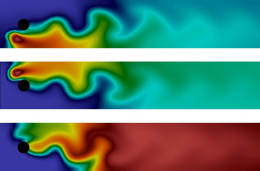
The solution at the final time is shown in Figure 11. We clearly see the advection of the species $ A $ and $ B $ and the formation of $ C $ along the center of the channel where $ A $ and $ B $ meet.

Figure 11: Plot of the concentrations of the three species $ A $, $ B $, and $ C $ (from top to bottom) at final time.

The complete code is presented below.

from fenics import *

T = 5.0            # final time
num_steps = 500    # number of time steps
dt = T / num_steps # time step size
eps = 0.01         # diffusion coefficient
K = 10.0           # reaction rate

# Read mesh from file
mesh = Mesh('navier_stokes_cylinder/cylinder.xml.gz')

# Define function space for velocity
W = VectorFunctionSpace(mesh, 'P', 2)

# Define function space for system of concentrations
P1 = FiniteElement('P', triangle, 1)
element = MixedElement([P1, P1, P1])
V = FunctionSpace(mesh, element)

# Define test functions
v_1, v_2, v_3 = TestFunctions(V)

# Define functions for velocity and concentrations
w = Function(W)
u = Function(V)
u_n = Function(V)

# Split system functions to access components
u_1, u_2, u_3 = split(u)
u_n1, u_n2, u_n3 = split(u_n)

# Define source terms
f_1 = Expression('pow(x[0]-0.1,2)+pow(x[1]-0.1,2)<0.05*0.05 ? 0.1 : 0',
                 degree=1)
f_2 = Expression('pow(x[0]-0.1,2)+pow(x[1]-0.3,2)<0.05*0.05 ? 0.1 : 0',
                 degree=1)
f_3 = Constant(0)

# Define expressions used in variational forms
k = Constant(dt)
K = Constant(K)
eps = Constant(eps)

# Define variational problem
F = ((u_1 - u_n1) / k)*v_1*dx + dot(w, grad(u_1))*v_1*dx \ 
  + eps*dot(grad(u_1), grad(v_1))*dx + K*u_1*u_2*v_1*dx  \ 
  + ((u_2 - u_n2) / k)*v_2*dx + dot(w, grad(u_2))*v_2*dx \ 
  + eps*dot(grad(u_2), grad(v_2))*dx + K*u_1*u_2*v_2*dx  \ 
  + ((u_3 - u_n3) / k)*v_3*dx + dot(w, grad(u_3))*v_3*dx \ 
  + eps*dot(grad(u_3), grad(v_3))*dx - K*u_1*u_2*v_3*dx + K*u_3*v_3*dx \ 
  - f_1*v_1*dx - f_2*v_2*dx - f_3*v_3*dx

# Create time series for reading velocity data
timeseries_w = TimeSeries('navier_stokes_cylinder/velocity_series')

# Create VTK files for visualization output
vtkfile_u_1 = File('reaction_system/u_1.pvd')
vtkfile_u_2 = File('reaction_system/u_2.pvd')
vtkfile_u_3 = File('reaction_system/u_3.pvd')

# Create progress bar
progress = Progress('Time-stepping')
set_log_level(PROGRESS)

# Time-stepping
t = 0
for n in range(num_steps):

    # Update current time
    t += dt

    # Read velocity from file
    timeseries_w.retrieve(w.vector(), t)

    # Solve variational problem for time step
    solve(F == 0, u)

    # Save solution to file (VTK)
    _u_1, _u_2, _u_3 = u.split()
    vtkfile_u_1 << (_u_1, t)
    vtkfile_u_2 << (_u_2, t)
    vtkfile_u_3 << (_u_3, t)

    # Update previous solution
    u_n.assign(u)

    # Update progress bar
    progress.update(t / T)

# Hold plot
interactive()

This example program can be found in the file ft09_reaction_system.py.

Finally, we comment on three important techniques that are very useful when working with systems of PDEs: setting initial conditions, setting boundary conditions, and extracting components of the system for plotting or postprocessing.

Setting initial conditions for mixed systems

In our example, we did not need to worry about setting an initial condition, since we start with $ u_1 = u_2 = u_3 = 0 $. This happens automatically in the code when we set u_n = Function(V). This creates a Function for the whole system and all degrees of freedom are set to zero.

If we want to set initial conditions for the components of the system separately, the easiest solution is to define the initial conditions as a vector-valued Expression and then project (or interpolate) this to the Function representing the whole system. For example,

u_0 = Expression(('sin(x[0])', 'cos(x[0]*x[1])', 'exp(x[1])'), degree=1)
u_n = project(u_0, V)

This defines $ u_1 $, $ u_2 $, and $ u_2 $ to be the projections of $ \sin x $, $ \cos (xy) $, and $ \exp(y) $, respectively.

Setting boundary conditions for mixed systems

In our example, we also did not need to worry about setting boundary conditions since we used a natural Neumann condition. If we want to set Dirichlet conditions for individual components of the system, this can be done as usual by the class DirichletBC, but we must specify for which subsystem we set the boundary condition. For example, to specify that $ u_2 $ should be equal to $ xy $ on the boundary defined by boundary, we do

u_D = Expression('x[0]*x[1]', degree=1)
bc = DirichletBC(V.sub(1), u_D, boundary)

The object bc or a list of such objects containing different boundary conditions, can then be passed to the solve function as usual. Note that numbering starts at $ 0 $ in FEniCS so the subspace corresponding to $ u_2 $ is V.sub(1).

Accessing components of mixed systems

If u is a Function defined on a mixed function space in FEniCS, there are several ways in which u can be split into components. Above we already saw an example of the first of these:

u_1, u_2, u_3 = split(u)

This extracts the components of u as symbols that can be used in a variational problem. The above statement is in fact equivalent to

u_1 = u[0]
u_2 = u[1]
u_3 = u[2]

Note that u[0] is not really a Function object, but merely a symbolic expression, just like grad(u) in FEniCS is a symbolic expression and not a Function representing the gradient. This means that u_1, u_2, u_3 can be used in a variational problem, but cannot be used for plotting or postprocessing.

To access the components of u for plotting and saving the solution to file, we need to use a different variant of the split function:

u_1_, u_2_, u_3_ = u.split()

This returns three subfunctions as actual objects with access to the common underlying data stored in u, which makes plotting and saving to file possible. Alternatively, we can do

u_1_, u_2_, u_3_ = u.split(deepcopy=True)

which will create u_1_, u_2_, and u_3_ as stand-alone Function objects, each holding a copy of the subfunction data extracted from u. This is useful in many situations but is not necessary for plotting and saving solutions to file.