Wave propagation from a source point

Question

Hello,
I am trying to model a wave propagating in a rectangular domain due to a source point located on the left edge of the rectangle. I am going to explain it more in some steps:

1- Wave Equation
The wave equation in two dimensions is defined as:

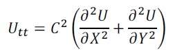
C: Wave Speed
2- Driving the weak forms equations
We have to drive the weak forms of the wave equation to implement it in a Finite Element code. First,we need to discretize the wave equation in time:

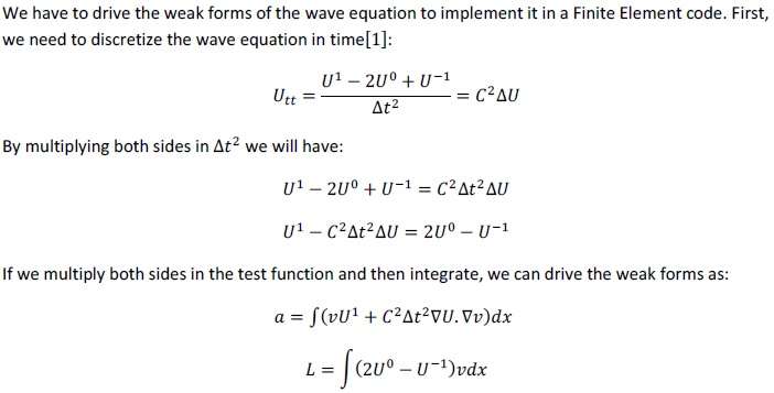
The domain is a rectangular 4 × 2 plate.
3) Initial and boundary conditions
Initial conditions are all zero. For boundary conditions, I want to put a source point on the left edge with an equation like:
U(t)=50 sin (25*t) and all of the initial conditions are zero.
4- Results
I took 3 snap shots of the start , middle and the end of the time period of this wave propagation.

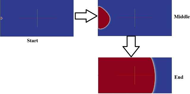
The thing is when we simulate a wave from a source point in another software like COMSOL, the propagating wave is shown in a different way:

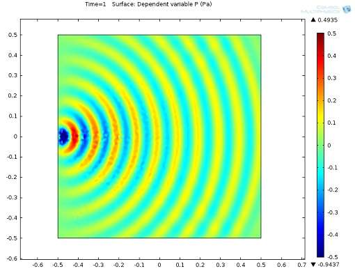
What I am trying to say is that there are for example blue lines and red lines next together but what I get from FEniCS (Paraview) does not even look like a wave propagation from a source point. Do you happen to know why it is like that and how I can get a correct animation? I think there might be something wrong with the modeling of the source point.
In addition, I have attached my final code.
Once thanks again for your time to answer my questions.

Code:

from dolfin import *
import numpy as np
c=5000
mesh = RectangleMesh(Point(-2,-1), Point(2,1),160,80)
V=FunctionSpace(mesh, "Lagrange", 1)

Time variables

dt = 0.000004; t = 0; T = 0.0004
init="0"
g = Expression(init,t=0)

Previous and current solution

u1= interpolate(g, V)
u0= interpolate(g, V)

Variational problem at each time

u = TrialFunction(V)
v = TestFunction(V)
a = uvdx + dtdtccinner(grad(u), grad(v))dx
L = 2u1vdx-u0vdx
bc = DirichletBC(V, 0,"on_boundary")
A, b = assemble_system(a, L, bc)
f = File("wave.pvd")
u=Function(V)

SourePoint definition & Solve

while t <= T:
b = assemble(L)
bc.apply(b)
delta = PointSource(V, Point(-2., 0.,), 50sin(25t))
delta.apply(b)
solve(A, u.vector(), b)
u0.assign(u1)
u1.assign(u)
t += dt
plot(u, interactive=False)
f<<u

Answer 1

Seems like your code is correct, but the frequency of your source function is too low. I was able to get something similar to your non-fenics solution by using the following code:

from dolfin import *
import numpy as np
c=5000
mesh = RectangleMesh(-2, -2, 2, 2,80,80)
V=FunctionSpace(mesh, "Lagrange", 1)

# Time variables
dt = 0.000004; t = 0; T = 0.004

# Previous and current solution
u1= interpolate(Constant(0.0), V)
u0= interpolate(Constant(0.0), V)

# Variational problem at each time
u = TrialFunction(V)
v = TestFunction(V)

a = u*v*dx + dt*dt*c*c*inner(grad(u), grad(v))*dx
L = 2*u1*v*dx-u0*v*dx

bc = DirichletBC(V, 0, "on_boundary")
A, b = assemble_system(a, L, bc)

u=Function(V)
while t <= T:
    A, b = assemble_system(a, L, bc)
    delta = PointSource(V, Point(-2.0, 0), sin(c * 10 * t))
    delta.apply(b)
    solve(A, u.vector(), b)
    u0.assign(u1)
    u1.assign(u)
    t += dt

    # Reduce the range of the solution so that we can see the waves
    j = 0
    for i in u.vector():
        i = min(.01, i)
        i = max(-.01, i)
        u.vector()[j] = i;
        j += 1

    plot(u, interactive=False)

plot(u, interactive=True)

Best,

Artur