7. Stokes equations with Mini elements
This demo is implemented in a single Python file,
demo_stokes-mini.py, which contains both the variational
form and the solver.
This demo illustrates how to:
- Read mesh and subdomains from file
- Use mixed function spaces
- Use enriched function spaces
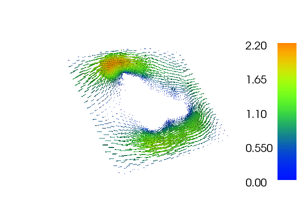
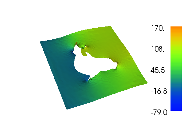
The solution for \(u\) and \(p\) in this demo will look as follows:
7.1. Equation and problem definition
Strong formulation:
Note
The sign of the pressure has been flipped from the classical definition. This is done in order to have a symmetric (but not positive-definite) system of equations rather than a non-symmetric (but positive-definite) system of equations.
A typical set of boundary conditions on the boundary \(\partial \Omega = \Gamma_{D} \cup \Gamma_{N}\) can be:
The Stokes equations can easily be formulated in a mixed variational form; that is, a form where the two variables, the velocity and the pressure, are approximated simultaneously. Using the abstract framework, we have the problem: find \((u, p) \in W\), such that
for all \((v, q) \in W\), where
The space \(W\) should be a mixed (product) function space: \(W = V \times Q\) such that \(u \in V \, {\rm and} \, q \in Q\).
In this demo, we shall consider the following definitions of the input functions, the domain, and the boundaries:
- \(\Omega = [0,1]\times[0, 1] \backslash {\rm dolphin}\) (a unit square)
- \(\Gamma_D =\)
- \(\Gamma_N =\)
- \(u_0 = (- \sin(\pi x_1), 0.0) \, {\rm for} \, x_0 = 1 \, {\rm and} \, u_0 = (0.0, 0.0)\) otherwise
- \(f = (0.0, 0.0)\)
- \(g = (0.0, 0.0)\)
7.2. Implementation
This description goes through the implementation (in
demo_stokes-mini.py) of a solver for the Stokes equation
step-by-step.
First, the dolfin module is imported:
from dolfin import *
In this example, different boundary conditions are prescribed on
different parts of the boundaries. This information must be made
available to the solver. One way of doing this, is to tag the
different sub-regions with different (integer) labels. DOLFIN provides
a class MeshFunction which
is useful for these types of operations: instances of this class
represent a functions over mesh entities (such as over cells or over
facets). Mesh and mesh functions can be read from file in the
following way:
# Load mesh and subdomains
mesh = Mesh("../dolfin_fine.xml.gz")
sub_domains = MeshFunction("size_t", mesh, "../dolfin_fine_subdomains.xml.gz")
Next, we define a FunctionSpace on Mini element
(P1 + B) * Q. UFL object P1 + B stands for the vectorial
Lagrange element of degree 1 enriched with the cubic Bubble.
(P1 + B) * Q defines the mixed element for velocity and pressure.
# Build function spaces on Mini element
P1 = VectorElement("Lagrange", mesh.ufl_cell(), 1)
B = VectorElement("Bubble",   mesh.ufl_cell(), 3)
Q = FiniteElement("Lagrange", mesh.ufl_cell(), 1)
W = FunctionSpace(mesh, (P1 + B) * Q)
Now that we have our mixed function space and marked subdomains defining the boundaries, we define boundary conditions:
# No-slip boundary condition for velocity
# NOTE: Projection here is inefficient workaround of issue #489, FFC issue #69
noslip = project(Constant((0, 0)), W.sub(0).collapse())
bc0 = DirichletBC(W.sub(0), noslip, sub_domains, 0)

# Inflow boundary condition for velocity
# NOTE: Projection here is inefficient workaround of issue #489, FFC issue #69
inflow = project(Expression(("-sin(x[1]*pi)", "0.0"), degree=2), W.sub(0).collapse())
bc1 = DirichletBC(W.sub(0), inflow, sub_domains, 1)

# Collect boundary conditions
bcs = [bc0, bc1]
Here, we have given four arguments in the call of
DirichletBC. The first
specifies the FunctionSpace. Since we have a
mixed function space, we write
W.sub(0) for the velocity componenet of the space,
and W.sub(1) for the pressure component of the space. The second
argument specifies the value on the Dirichlet boundary. The two last
arguments specify the marking of the subdomains; sub_domains contains
the subdomain markers and the number given as the last argument is the
subdomain index.
The bilinear and linear forms corresponding to the weak mixed formulation of the Stokes equations are defined as follows:
# Define variational problem
(u, p) = TrialFunctions(W)
(v, q) = TestFunctions(W)
f = Constant((0, 0))
a = (inner(grad(u), grad(v)) - div(v)*p + q*div(u))*dx
L = inner(f, v)*dx
To compute the solution we use the bilinear and linear forms, and the
boundary condition, but we also need to create a Function to store the solution(s). The (full)
solution will be stored in w, which we initialize using the mixed
function space W. The actual
computation is performed by calling solve with the arguments a,
L, w and bcs. The separate components u and p of
the solution can be extracted by calling the split function. Here we use an
optional argument True in the split function to specify that we want a
deep copy. If no argument is given we will get a shallow copy. We want
a deep copy for further computations on the coefficient vectors.
# Compute solution
w = Function(W)
solve(a == L, w, bcs)

# Split the mixed solution using deepcopy
# (needed for further computation on coefficient vector)
(u, p) = w.split(True)
We may be interested in the \(l^2\) norms of u and p, they can be calculated and printed by writing
print("Norm of velocity coefficient vector: %.15g" % u.vector().norm("l2"))
print("Norm of pressure coefficient vector: %.15g" % p.vector().norm("l2"))
One can also split functions using shallow copies (which is enough when we just plot the result) by writing
# Split the mixed solution using a shallow copy
(u, p) = w.split()
Finally, we can store to file and plot the solutions.
# Save solution in VTK format
ufile_pvd = File("velocity.pvd")
ufile_pvd << u
pfile_pvd = File("pressure.pvd")
pfile_pvd << p

# Plot solution
plot(u)
plot(p)
interactive()
7.3. Complete code
from __future__ import print_function
from dolfin import *

# Load mesh and subdomains
mesh = Mesh("../dolfin_fine.xml.gz")
sub_domains = MeshFunction("size_t", mesh, "../dolfin_fine_subdomains.xml.gz")

# Build function spaces on Mini element
P1 = VectorElement("Lagrange", mesh.ufl_cell(), 1)
B = VectorElement("Bubble",   mesh.ufl_cell(), 3)
Q = FiniteElement("Lagrange", mesh.ufl_cell(), 1)
W = FunctionSpace(mesh, (P1 + B) * Q)

# No-slip boundary condition for velocity
# NOTE: Projection here is inefficient workaround of issue #489, FFC issue #69
noslip = project(Constant((0, 0)), W.sub(0).collapse())
bc0 = DirichletBC(W.sub(0), noslip, sub_domains, 0)

# Inflow boundary condition for velocity
# NOTE: Projection here is inefficient workaround of issue #489, FFC issue #69
inflow = project(Expression(("-sin(x[1]*pi)", "0.0"), degree=2), W.sub(0).collapse())
bc1 = DirichletBC(W.sub(0), inflow, sub_domains, 1)

# Collect boundary conditions
bcs = [bc0, bc1]

# Define variational problem
(u, p) = TrialFunctions(W)
(v, q) = TestFunctions(W)
f = Constant((0, 0))
a = (inner(grad(u), grad(v)) - div(v)*p + q*div(u))*dx
L = inner(f, v)*dx

# Compute solution
w = Function(W)
solve(a == L, w, bcs)

# Split the mixed solution using deepcopy
# (needed for further computation on coefficient vector)
(u, p) = w.split(True)

print("Norm of velocity coefficient vector: %.15g" % u.vector().norm("l2"))
print("Norm of pressure coefficient vector: %.15g" % p.vector().norm("l2"))

# Split the mixed solution using a shallow copy
(u, p) = w.split()

# Save solution in VTK format
ufile_pvd = File("velocity.pvd")
ufile_pvd << u
pfile_pvd = File("pressure.pvd")
pfile_pvd << p

# Plot solution
plot(u)
plot(p)
interactive()