21. Tensor-weighted Poisson¶

This demo is implemented in two files; one file, generate_data.py , for generating data, and one file, demo_tensor-weighted-poisson.py , which contains both the vaiational form and the solver.

This demo illustrates how to

Import data from file
Use complex user-defined JIT-compiled expressions

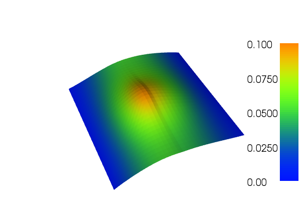
The solution \(u\) will look like this

../../../../_images/tensorweighted-poisson_u.png

21.1. Equation and problem definition¶

The Poisson equation is the canonical elliptic partial differential equation. For a domain \(\Omega \subset \mathbb{R}^n\) with boundary \(\partial \Omega = \Gamma_{D} \cup \Gamma_{N}\), the Poisson equation with variational conductivity \(C\) and particular boundary conditions reads:

\[\begin{split}- \nabla \cdot (C \nabla u) &= f \quad {\rm in} \ \Omega, \\ u &= 0 \quad {\rm on} \ \Gamma_{D}, \\ \frac{\partial u}{\partial n} &= 0 \quad {\rm on} \ \Gamma_{N}. \\\end{split}\]

Here, \(f\) is input data and \(n\) denotes the outward directed boundary normal. The variational form of the Poisson equation reads: find \(u \in V\) such that

\[a(u, v) = L(v) \quad \forall \ v \in V,\]

where \(V\) is a suitable function space and

\[\begin{split}a(u, v) &= \int_{\Omega} C \nabla u \cdot \nabla v \, {\rm d} x, \\ L(v) &= \int_{\Omega} f v \, {\rm d} x.\end{split}\]

The expression \(a(u, v)\) is the bilinear form and \(L(v)\) is the linear form. It is assumed that all functions in \(V\) satisfy the Dirichlet boundary conditions (\(u = 0 \ {\rm on} \Gamma_{D}\)).

In this demo, we shall consider the following definitions of the domain, the boundaries and the input function:

\(\Omega = [0,1] \times [0,1]\) (a unit square)
\(\Gamma_{D} = \{(0, y) \cup (1, y) \subset \partial \Omega\}\) (Dirichlet boundary)
\(\Gamma_{N} = \{(x, 0) \cup (x, 1) \subset \partial \Omega\}\) (Neumann boundary)
\(f = 10\exp(-((x - 0.5)^2 + (y - 0.5)^2) / 0.02)\) (source term).

The conductivity is a symmetric \(2 \times 2\) matrix which varies throughout the domain. In the left part of the domain the conductivity is

\[\begin{split}C = \begin{bmatrix} 1 & 0.3 \\ 0.3 & 2 \end{bmatrix}\end{split}\]

and in the right part it is

\[\begin{split}C = \begin{bmatrix} 3 & 0.5 \\ 0.5 & 4 \end{bmatrix}.\end{split}\]

21.2. Implementation¶

21.2.1. Implementation of generate_data.py¶

First, the dolfin module is imported:

from dolfin import *

Then, we define a mesh of the domain. We use the built-in mesh, provided by the class UnitSquareMesh. In order to create a mesh consisting of \(32 \times 32\) squares with each square divided into two triangles, we do as follows:

# Create mesh
mesh = UnitSquareMesh(32, 32)

Now, we create mesh functions to store the values of the conductivity matrix as it varies over the domain. Since the matrix is symmetric, we only create mesh functions for the upper triangular part of the matrix. In MeshFunction the first argument specifies the type of the mesh function, here we use “double”. Other types allowed are “int”, “size_t” and “bool”. The two following arguments are optional; the first gives the mesh the MeshFunction is defined on, and the second the topological dimension of the mesh function.

# Create mesh functions for c00, c01, c11
c00 = MeshFunction("double", mesh, 2)
c01 = MeshFunction("double", mesh, 2)
c11 = MeshFunction("double", mesh, 2)

To set the values of the mesh functions, we go through all the cells in the mesh and check whether the midpoint value of the cell in the \(x\)-direction is less than 0.5 or not (in practice this means that we are checking which half of the unit square the cell is in). Then we set the correct values of the mesh functions, depending on which half we are in.

# Iterate over mesh and set values
for cell in cells(mesh):
    if cell.midpoint().x() < 0.5:
        c00[cell] = 1.0
        c01[cell] = 0.3
        c11[cell] = 2.0
    else:
        c00[cell] = 3.0
        c01[cell] = 0.5
        c11[cell] = 4.0

Create files to store data and save to file:

# Store to file
mesh_file = File("../unitsquare_32_32.xml.gz")
c00_file = File("../unitsquare_32_32_c00.xml.gz")
c01_file = File("../unitsquare_32_32_c01.xml.gz")
c11_file = File("../unitsquare_32_32_c11.xml.gz")

mesh_file << mesh
c00_file << c00
c01_file << c01
c11_file << c11

Plot the mesh functions using the plot function:

# Plot mesh functions
plot(c00, title="C00")
plot(c01, title="C01")
plot(c11, title="C11")

interactive()

21.2.2. Implementation of tensor-weighted-poisson.py¶

This description goes through the implementation (in demo_tensor-weighted-poisson.py ) of a solver for the above described Poisson equation step-by-step.

First, the dolfin module is imported:

from dolfin import *

We proceed by defining a mesh of the domain and a finite element function space \(V\) relative to this mesh. We read the mesh file generated by generate_data.py and create the function space in the following way:

# Read mesh from file and create function space
mesh = Mesh("../unitsquare_32_32.xml.gz")
V = FunctionSpace(mesh, "Lagrange", 1)

The second argument to FunctionSpace is the finite element family, while the third argument specifies the polynomial degree. Thus, in this case, our space V consists of first-order, continuous Lagrange finite element functions (or in order words, continuous piecewise linear polynomials).

Next, we want to consider the Dirichlet boundary condition. A simple Python function, returning a boolean, can be used to define the subdomain for the Dirichlet boundary condition (\(\Gamma_D\)). The function should return True for those points inside the subdomain and False for the points outside. In our case, we want to say that the points \((x, y)\) such that \(x = 0\) or \(x = 1\) are inside on the inside of \(\Gamma_D\). (Note that because of rounding-off errors, it is often wise to instead specify \(x < \epsilon\) or \(x > 1 - \epsilon\) where \(\epsilon\) is a small number (such as machine precision).)

# Define Dirichlet boundary (x = 0 or x = 1)
def boundary(x):
    return x[0] < DOLFIN_EPS or x[0] > 1.0 - DOLFIN_EPS

Now, the Dirichlet boundary condition can be created using the class DirichletBC. A DirichletBC takes three arguments: the function space the boundary condition applies to, the value of the boundary condition, and the part of the boundary on which the condition applies. In our example, the function space is \(V\). The value of the boundary condition \((0.0)\) can be represented using a Constant and the Dirichlet boundary is defined immediately above. The definition of the Dirichlet boundary condition then looks as follows:

# Define boundary condition
u0 = Constant(0.0)
bc = DirichletBC(V, u0, boundary)

Before we define the conductivity matrix, we create a string containing C++ code for evaluation of the conductivity. Later we will use this string when we create an Expression containing the entries of the matrix.

# Code for C++ evaluation of conductivity
conductivity_code = """

class Conductivity : public Expression
{
public:

  // Create expression with 3 components
  Conductivity() : Expression(3) {}

  // Function for evaluating expression on each cell
  void eval(Array<double>& values, const Array<double>& x, const ufc::cell& cell) const
  {
    const uint D = cell.topological_dimension;
    const uint cell_index = cell.index;
    values[0] = (*c00)[cell_index];
    values[1] = (*c01)[cell_index];
    values[2] = (*c11)[cell_index];
  }

  // The data stored in mesh functions
  std::shared_ptr<MeshFunction<double> > c00;
  std::shared_ptr<MeshFunction<double> > c01;
  std::shared_ptr<MeshFunction<double> > c11;

};
"""

We define the conductivity matrix by first creating mesh functions from the files we stored in generate_data.py. Here, the third argument in MeshFunction is the path to the data files. Then, we define an expression for the entries in the matrix where we give the C++ code as an argument for optimalization. Finally, we use the UFL function as_matrix to create the matrix consisting of the expressions.

# Define conductivity expression and matrix
c00 = MeshFunction("double", mesh, "../unitsquare_32_32_c00.xml.gz")
c01 = MeshFunction("double", mesh, "../unitsquare_32_32_c01.xml.gz")
c11 = MeshFunction("double", mesh, "../unitsquare_32_32_c11.xml.gz")

c = Expression(cppcode=conductivity_code, degree=0)
c.c00 = c00
c.c01 = c01
c.c11 = c11
C = as_matrix(((c[0], c[1]), (c[1], c[2])))

Next, we want to express the variational problem. First, we need to specify the trial function \(u\) and the test function \(v\), both living in the function space \(V\). We do this by defining a TrialFunction and a TestFunction on the previously defined FunctionSpace \(V\).

Further, the source \(f\) is involved in the variational form, and hence it must be must specified. Since \(f\) is given by a simple mathematical formula, it can easily be declared using the Expression class. Note that the string defining \(f\) uses C++ syntax since, for efficiency, DOLFIN will generate and compile C++ code for these expressions at run-time.

With these ingredients, we can write down the bilinear form \(a\) and the linear form \(L\) (using UFL operators). In summary, this reads:

# Define variational problem
u = TrialFunction(V)
v = TestFunction(V)
f = Expression("10*exp(-(pow(x[0] - 0.5, 2) + pow(x[1] - 0.5, 2)) / 0.02)", degree=2)
a = inner(C*grad(u), grad(v))*dx
L = f*v*dx

Now, we have specified the bilinear and linear forms and can consider the solution of the variational problem. First, we need to define a Function u to represent the solution. (Upon initialization, it is simply set to the zero function.) A Function represents a function living in a finite element function space. Next, we can call the solve function with the arguments a == L, u and bc as follows:

# Compute solution
u = Function(V)
solve(a == L, u, bc)

The function u will be modified during the call to solve. The default settings for solving a variational problem have been used. However, the solution process can be controlled in much more detail if desired.

A Function can be manipulated in various ways, in particular, it can be plotted and saved to file. Here, we output the solution to a VTK file (using the suffix .pvd) for later visualization and also plot it using the plot command:

# Save solution in VTK format
file = File("poisson.pvd")
file << u

# Plot solution
plot(u, interactive=True)

21.3. Complete code¶

demo_tensor-weighted-poisson.py:

from dolfin import *

# Read mesh from file and create function space
mesh = Mesh("../unitsquare_32_32.xml.gz")
V = FunctionSpace(mesh, "Lagrange", 1)

# Define Dirichlet boundary (x = 0 or x = 1)
def boundary(x):
    return x[0] < DOLFIN_EPS or x[0] > 1.0 - DOLFIN_EPS

# Define boundary condition
u0 = Constant(0.0)
bc = DirichletBC(V, u0, boundary)

# Code for C++ evaluation of conductivity
conductivity_code = """

class Conductivity : public Expression
{
public:

  // Create expression with 3 components
  Conductivity() : Expression(3) {}

  // Function for evaluating expression on each cell
  void eval(Array<double>& values, const Array<double>& x, const ufc::cell& cell) const
  {
    const uint D = cell.topological_dimension;
    const uint cell_index = cell.index;
    values[0] = (*c00)[cell_index];
    values[1] = (*c01)[cell_index];
    values[2] = (*c11)[cell_index];
  }

  // The data stored in mesh functions
  std::shared_ptr<MeshFunction<double> > c00;
  std::shared_ptr<MeshFunction<double> > c01;
  std::shared_ptr<MeshFunction<double> > c11;

};
"""

# Define conductivity expression and matrix
c00 = MeshFunction("double", mesh, "../unitsquare_32_32_c00.xml.gz")
c01 = MeshFunction("double", mesh, "../unitsquare_32_32_c01.xml.gz")
c11 = MeshFunction("double", mesh, "../unitsquare_32_32_c11.xml.gz")

c = Expression(cppcode=conductivity_code, degree=0)
c.c00 = c00
c.c01 = c01
c.c11 = c11
C = as_matrix(((c[0], c[1]), (c[1], c[2])))

# Define variational problem
u = TrialFunction(V)
v = TestFunction(V)
f = Expression("10*exp(-(pow(x[0] - 0.5, 2) + pow(x[1] - 0.5, 2)) / 0.02)", degree=2)
a = inner(C*grad(u), grad(v))*dx
L = f*v*dx

# Compute solution
u = Function(V)
solve(a == L, u, bc)

# Save solution in VTK format
file = File("poisson.pvd")
file << u

# Plot solution
plot(u, interactive=True)

generate_data.py:

from dolfin import *

# Create mesh
mesh = UnitSquareMesh(32, 32)

# Create mesh functions for c00, c01, c11
c00 = MeshFunction("double", mesh, 2)
c01 = MeshFunction("double", mesh, 2)
c11 = MeshFunction("double", mesh, 2)

# Iterate over mesh and set values
for cell in cells(mesh):
    if cell.midpoint().x() < 0.5:
        c00[cell] = 1.0
        c01[cell] = 0.3
        c11[cell] = 2.0
    else:
        c00[cell] = 3.0
        c01[cell] = 0.5
        c11[cell] = 4.0

# Store to file
mesh_file = File("../unitsquare_32_32.xml.gz")
c00_file = File("../unitsquare_32_32_c00.xml.gz")
c01_file = File("../unitsquare_32_32_c01.xml.gz")
c11_file = File("../unitsquare_32_32_c11.xml.gz")

mesh_file << mesh
c00_file << c00
c01_file << c01
c11_file << c11

# Plot mesh functions
plot(c00, title="C00")
plot(c01, title="C01")
plot(c11, title="C11")

interactive()